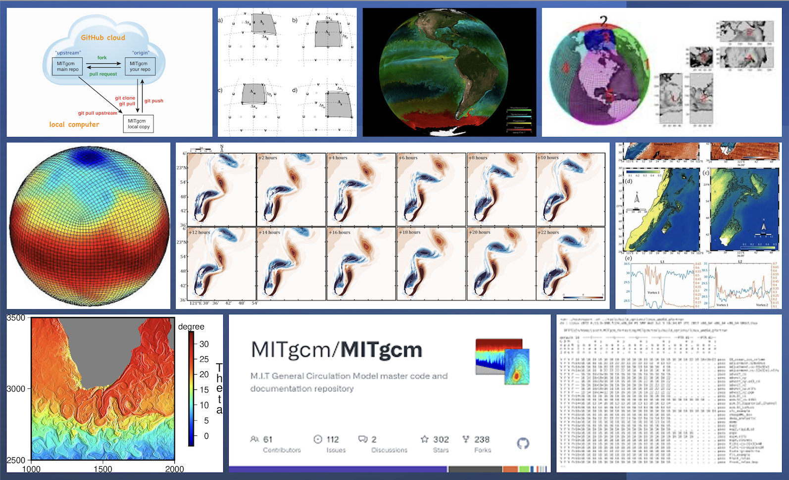
MITgcm
A numerical model designed for study of the atmosphere, ocean, and climate, MITgcm’s flexible non-hydrostatic formulation enables it to efficiently simulate fluid phenomena over a wide range of scales; its adjoint capabilities enable it to be applied to sensitivity questions and to parameter and state estimation problems. By employing fluid equation isomorphisms, a single dynamical kernel can be used to simulate flow of both the atmosphere and ocean. The model is developed to perform efficiently on a wide variety of computational platforms.

2023 Research Roundup
Happy 2024: Another new year, another new research roundup! Best wishes as always to MITgcmers past, MITgcmers present and MITgcmers yet to come…
Exploring the effects of optimizing model-dependent parameters on Antarctic sea-ice concentration data assimilation
Improving the performance of the Data Assimilation System for the Southern Ocean in assimilating sea-ice concentration (SIC) through optimizing model-dependent parameters.
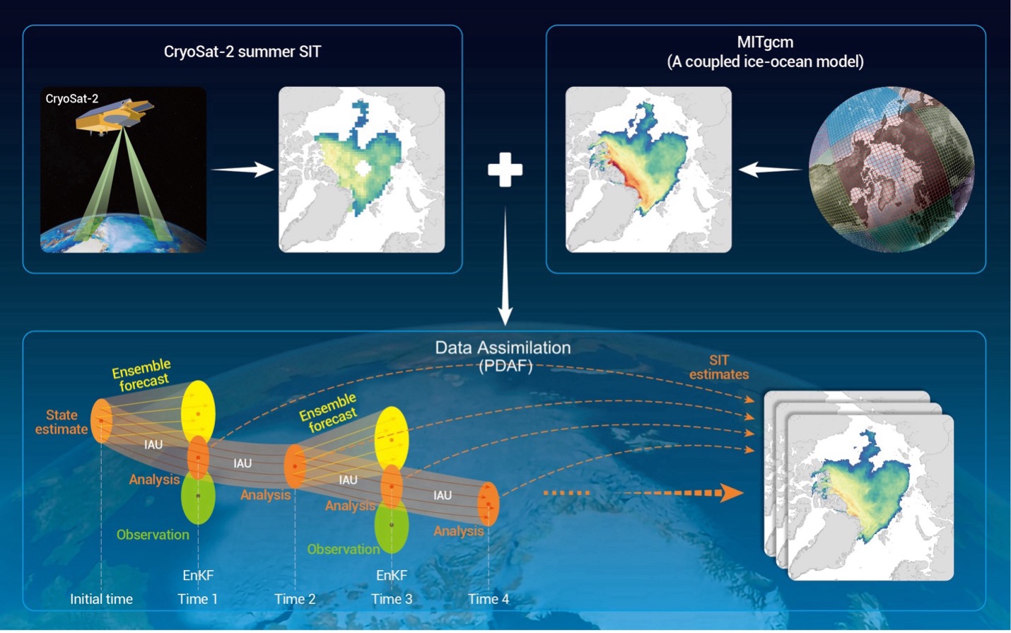
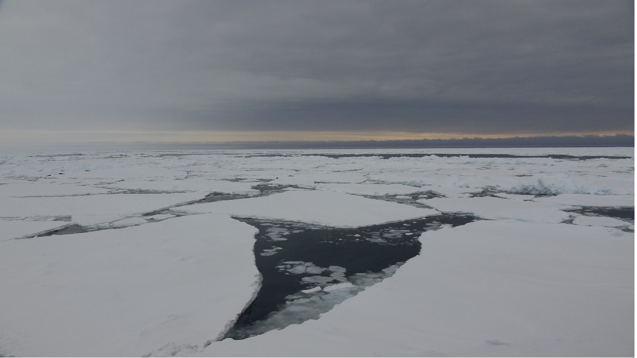
Assimilating CryoSat-2 Summer Sea Ice Thickness Observations
By incorporating satellite observations of summer sea ice thickness and concentration into MITgcm., a team of researchers from China and Germany is helping improve Arctic summer sea ice thickness estimation.
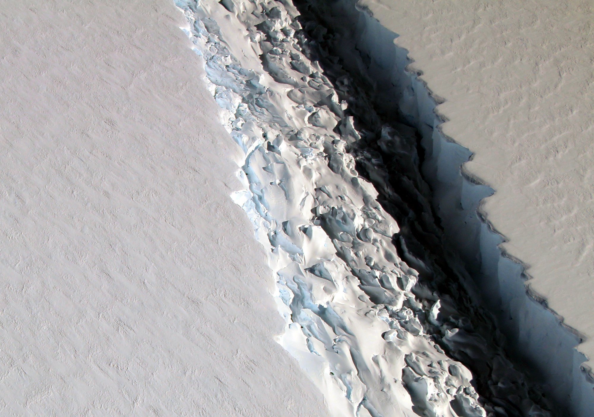
Antarctic Rifts and Icebergs
Mattia Poinelli uses MITgcm to explore what role rifts and icebergs play in shaping the dynamics of Antarctic ice shelves.
Subglacial Melting
This month we spotlight research using a regional implementation of MITgcm to explore Antarctic subglacial runoff.

MITgcm goes to EGU
This month, a taste from the blizzard of papers using MITgcm served up at the European Geophysical Union General Assembly this year.