Home Contact Us Site Map  
 
       
    next up previous contents
Next: 6.3.2 GM parameterization Up: 6.3 Gent/McWiliams/Redi SGS Eddy Previous: 6.3 Gent/McWiliams/Redi SGS Eddy   Contents

6.3.1 Redi scheme: Isopycnal diffusion

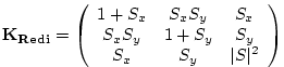
The Redi scheme diffuses tracers along isopycnals and introduces a term in the tendency (rhs) of such a tracer (here $ \tau$) of the form:

$\displaystyle \bf {\nabla} \cdot \kappa_\rho \bf {K}_{Redi} \bf {\nabla} \tau$ (6.1)

where $ \kappa_\rho$ is the along isopycnal diffusivity and $ \bf {K}_{Redi}$ is a rank 2 tensor that projects the gradient of $ \tau$ onto the isopycnal surface. The unapproximated projection tensor is:

$\displaystyle \bf {K}_{Redi} = \left( \begin{array}{ccc} 1 + S_x& S_x S_y & S_x \\ S_x S_y & 1 + S_y & S_y \\ S_x & S_y & \vert S\vert^2 \\ \end{array} \right)$ (6.2)

Here, $ S_x = -\partial_x \sigma / \partial_z \sigma$ and $ S_y =
-\partial_y \sigma / \partial_z \sigma$ are the components of the isoneutral slope.

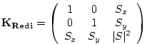
The first point to note is that a typical slope in the ocean interior is small, say of the order $ 10^{-4}$. A maximum slope might be of order $ 10^{-2}$ and only exceeds such in unstratified regions where the slope is ill defined. It is therefore justifiable, and customary, to make the small slope approximation, $ \vert S\vert << 1$. The Redi projection tensor then becomes:

$\displaystyle \bf {K}_{Redi} = \left( \begin{array}{ccc} 1 & 0 & S_x \\ 0 & 1 & S_y \\ S_x & S_y & \vert S\vert^2 \\ \end{array} \right)$ (6.3)


next up previous contents
Next: 6.3.2 GM parameterization Up: 6.3 Gent/McWiliams/Redi SGS Eddy Previous: 6.3 Gent/McWiliams/Redi SGS Eddy   Contents
mitgcm-support@dev.mitgcm.org
Copyright © 2002 Massachusetts Institute of Technology