|
|
|
|


Next: 3.13.3 Experiment Configuration
Up: 3.13 P coordinate Global
Previous: 3.13.1 Overview
Contents
Due to the pressure coordinate, the model can only be hydrostatic
[de Szoeke and Samelson, 2002]. The domain is discretized with a uniform grid
spacing in latitude and longitude on the sphere
 , so that there are ninety grid cells in the zonal
and forty in the meridional direction. The internal model coordinate
variables
, so that there are ninety grid cells in the zonal
and forty in the meridional direction. The internal model coordinate
variables  and
and  are initialized according to
Arctic polar regions are not included in this experiment. Meridionally
the model extends from
 to
to
 .
Vertically the model is configured with fifteen layers with the
following thicknesses
.
Vertically the model is configured with fifteen layers with the
following thicknesses
 |
 |
 Pa Pa |
|
 |
|
 Pa Pa |
|
 |
|
 Pa Pa |
|
 |
|
 Pa Pa |
|
 |
|
 Pa Pa |
|
 |
|
 Pa Pa |
|
 |
|
 Pa Pa |
|
 |
|
 Pa Pa |
|
 |
|
 Pa Pa |
|
 |
|
 Pa Pa |
|
 |
|
 Pa Pa |
|
 |
|
 Pa Pa |
|
 |
|
 Pa Pa |
|
 |
|
 Pa Pa |
|
 |
|
 Pa Pa |
|
(here the numeric subscript indicates the model level index number,
 ; note, that the surface layer has the highest index number 15) to
give a total depth,
; note, that the surface layer has the highest index number 15) to
give a total depth,  , of
, of
 . In pressure, this is
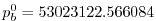 Pa
.
The implicit free surface form of the pressure equation described in
Marshall et al. [1997b] with the nonlinear extension by
Campin et al. [2004] is employed. A Laplacian operator, Pa
.
The implicit free surface form of the pressure equation described in
Marshall et al. [1997b] with the nonlinear extension by
Campin et al. [2004] is employed. A Laplacian operator,  , provides viscous
dissipation. Thermal and haline diffusion is also represented by a Laplacian operator.
, provides viscous
dissipation. Thermal and haline diffusion is also represented by a Laplacian operator.
Wind-stress forcing is added to the momentum equations in (3.55)
for both the zonal flow,  and the meridional flow
  , according to equations
(3.49) and (3.50).
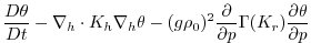
Thermodynamic forcing inputs are added to the equations
in (3.55) for
potential temperature,
, according to equations
(3.49) and (3.50).
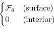
Thermodynamic forcing inputs are added to the equations
in (3.55) for
potential temperature,  , and salinity,
  , according to equations
(3.51) and (3.52).
This produces a set of equations solved in this configuration as follows:
, according to equations
(3.51) and (3.52).
This produces a set of equations solved in this configuration as follows:
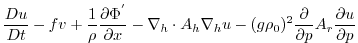 |
|
 |
(3.55) |
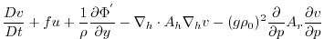 |
|
 |
(3.56) |
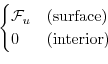
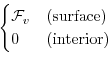
 |
|
0 |
(3.57) |
 |
|
 |
(3.58) |
 |
|
 |
(3.59) |
 |
|
 |
(3.60) |
where
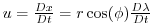 and
and
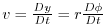 are the zonal and meridional
components of the flow vector,
are the zonal and meridional
components of the flow vector,  , on the sphere. As described
in MITgcm Numerical Solution Procedure 2, the
time evolution of potential temperature,
, equation is solved
prognostically. The full geopotential height,
, on the sphere. As described
in MITgcm Numerical Solution Procedure 2, the
time evolution of potential temperature,
, equation is solved
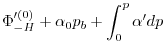
prognostically. The full geopotential height,  , is diagnosed by
summing the geopotential height anomalies
, is diagnosed by
summing the geopotential height anomalies  due to bottom
pressure
due to bottom
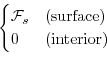
pressure  and density variations. The integration of the
hydrostatic equation is started at the bottom of the domain. The
condition of
and density variations. The integration of the
hydrostatic equation is started at the bottom of the domain. The
condition of  at the sea surface requires a time-independent
integration constant for the height anomaly due to density variations
at the sea surface requires a time-independent
integration constant for the height anomaly due to density variations
 , which is provided as an input field.
Next: 3.13.3 Experiment Configuration
Up: 3.13 P coordinate Global
Previous: 3.13.1 Overview
Contents
mitgcm-support@mitgcm.org
| Copyright © 2006
Massachusetts Institute of Technology |
Last update 2018-01-23 |
 |
|


