 |
 |
|||||||||||
 |
|
|||||||||||
 |
 |
|||||||||||


|
Next: 3.16.1 Configuration Up: 3. Getting Started with Previous: 3.15.6 Running the example Contents
|
![\includegraphics[width=\textwidth,height=.3\textheight]{s_examples/plume_on_slope/billows.eps}](img1584.png)
|
An important test of any ocean model is the ability to represent the flow of dense fluid down a slope. One example of such a flow is a non-rotating gravity plume on a continental slope, forced by a limited area of surface cooling above a continental shelf. Because the flow is non-rotating, a two dimensional model can be used in the across slope direction. The experiment is non-hydrostatic and uses open-boundaries to radiate transients at the deep water end. (Dense flow down a slope can also be forced by a dense inflow prescribed on the continental shelf; this configuration is being implemented by the DOME (Dynamics of Overflow Mixing and Entrainment) collaboration to compare solutions in different models). The files for this experiment can be found in the verification directory under tutorial_plume_on_slope.
The fluid is initially unstratified. The surface buoyancy loss ![]() (dimensions of L
(dimensions of L![]() T
T![]() ) over a cross-shelf distance
) over a cross-shelf distance ![]() causes
vertical convective mixing and modifies the density of the fluid by an
amount
causes
vertical convective mixing and modifies the density of the fluid by an
amount
| (3.80) |
where
 |
(3.81) |
A steady state is rapidly established in which the buoyancy flux out of the cooling region is balanced by the surface buoyancy loss. Then
| (3.82) |
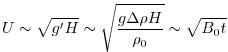
The Froude number of the flow on the shelf is close to unity (but in practice slightly less than unity, giving subcritical flow). When the flow reaches the slope, it accelerates, so that it may become supercritical (provided the slope angle
| (3.83) |
where
| (3.84) |
Finally, since we have assumed that the convective mixing on the shelf occurs in a much shorter time than the horizontal equilibration, this implies
Hence to summarize the important nondimensional parameters, and the limits we are considering:
| (3.85) |
In addition we are assuming that the slope is steep enough to provide sufficient acceleration to the gravity plume, but nonetheless much less that
Subsections
- 3.16.1 Configuration
- 3.16.2 Binary input data
- 3.16.3 Code configuration
- 3.16.4 Model parameters
- 3.16.5 Build and run the model
Next: 3.16.1 Configuration Up: 3. Getting Started with Previous: 3.15.6 Running the example Contents mitgcm-support@mitgcm.org
| Copyright © 2006 Massachusetts Institute of Technology | Last update 2018-01-23 |


