Home Contact Us Site Map  
 
       
    next up previous contents
Next: 2.15.1 Relative vorticity Up: 2. Discretization and Algorithm Previous: 2.14.8 Mom Diagnostics   Contents


2.15 Vector invariant momentum equations

The finite volume method lends itself to describing the continuity and tracer equations in curvilinear coordinate systems. However, in curvilinear coordinates many new metric terms appear in the momentum equations (written in Lagrangian or flux-form) making generalization far from elegant. Fortunately, an alternative form of the equations, the vector invariant equations are exactly that; invariant under coordinate transformations so that they can be applied uniformly in any orthogonal curvilinear coordinate system such as spherical coordinates, boundary following or the conformal spherical cube system.

The non-hydrostatic vector invariant equations read:

$\displaystyle \partial_t \vec{v} + ( 2\vec{\Omega} + \vec{\zeta}) \wedge \vec{v} - b \hat{r} + \vec{\nabla} B = \vec{\nabla} \cdot \vec{\bf\tau}$ (2.141)

which describe motions in any orthogonal curvilinear coordinate system. Here, $ B$ is the Bernoulli function and $ \vec{\zeta}=\nabla
\wedge \vec{v}$ is the vorticity vector. We can take advantage of the elegance of these equations when discretizing them and use the discrete definitions of the grad, curl and divergence operators to satisfy constraints. We can also consider the analogy to forming derived equations, such as the vorticity equation, and examine how the discretization can be adjusted to give suitable vorticity advection among other things.

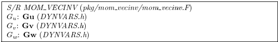
The underlying algorithm is the same as for the flux form equations. All that has changed is the contents of the ``G's''. For the time-being, only the hydrostatic terms have been coded but we will indicate the points where non-hydrostatic contributions will enter:

$\displaystyle G_u$ $\displaystyle =$ $\displaystyle G_u^{fv} + G_u^{\zeta_3 v} + G_u^{\zeta_2 w} + G_u^{\partial_x B}
+ G_u^{\partial_z \tau^x} + G_u^{h-dissip} + G_u^{v-dissip}$ (2.142)
$\displaystyle G_v$ $\displaystyle =$ $\displaystyle G_v^{fu} + G_v^{\zeta_3 u} + G_v^{\zeta_1 w} + G_v^{\partial_y B}
+ G_v^{\partial_z \tau^y} + G_v^{h-dissip} + G_v^{v-dissip}$ (2.143)
$\displaystyle G_w$ $\displaystyle =$ $\displaystyle G_w^{fu} + G_w^{\zeta_1 v} + G_w^{\zeta_2 u} + G_w^{\partial_z B}
+ G_w^{h-dissip} + G_w^{v-dissip}$ (2.144)

\fbox{ \begin{minipage}{4.75in}
{\em S/R MOM\_VECINV} ({\em pkg/mom\_vecinv/mom\...
...bf Gv} ({\em DYNVARS.h})
\par
$G_w$: {\bf Gw} ({\em DYNVARS.h})
\end{minipage} }


Subsections
next up previous contents
Next: 2.15.1 Relative vorticity Up: 2. Discretization and Algorithm Previous: 2.14.8 Mom Diagnostics   Contents
mitgcm-support@mitgcm.org
Copyright © 2006 Massachusetts Institute of Technology Last update 2018-01-23