 |
 |
|||||||||||
 |
|
|||||||||||
 |
 |
|||||||||||


|
Next: 2.17 Linear advection schemes Up: 2.16 Tracer equations Previous: 2.16 Tracer equations Contents
|
| (2.166) |
where
| (2.167) | |||
| (2.168) |
and the forcing can be some arbitrary function of state, time and space.
The term,
![]() , is required to retain local
conservation in conjunction with the linear implicit free-surface. It
only affects the surface layer since the flow is non-divergent
everywhere else. This term is therefore referred to as the surface
correction term. Global conservation is not possible using the
flux-form (as here) and a linearized free-surface
(Campin et al. [2004]; Griffies and Hallberg [2000]).
, is required to retain local
conservation in conjunction with the linear implicit free-surface. It
only affects the surface layer since the flow is non-divergent
everywhere else. This term is therefore referred to as the surface
correction term. Global conservation is not possible using the
flux-form (as here) and a linearized free-surface
(Campin et al. [2004]; Griffies and Hallberg [2000]).
The continuity equation can be recovered by setting
![]() and
and ![]() .
.
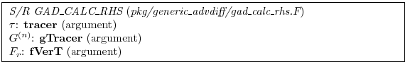
The driver routine that calls the routines to calculate tendencies are S/R CALC_GT and S/R CALC_GS for temperature and salt (moisture), respectively. These in turn call a generic advection diffusion routine S/R GAD_CALC_RHS that is called with the flow field and relevant tracer as arguments and returns the collective tendency due to advection and diffusion. Forcing is add subsequently in S/R CALC_GT or S/R CALC_GS to the same tendency array.
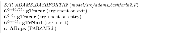
The space and time discretization are treated separately (method of
lines). Tendencies are calculated at time levels ![]() and
and ![]() and
extrapolated to
and
extrapolated to ![]() using the Adams-Bashforth method:
using the Adams-Bashforth method:
| (2.169) |
where
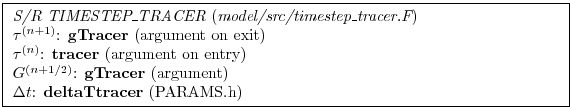
The tracers are stepped forward in time using the extrapolated tendency:
| (2.170) |
Strictly speaking the ABII scheme should be applied only to the advection terms. However, this scheme is only used in conjunction with the standard second, third and fourth order advection schemes. Selection of any other advection scheme disables Adams-Bashforth for tracers so that explicit diffusion and forcing use the forward method.
Next: 2.17 Linear advection schemes Up: 2.16 Tracer equations Previous: 2.16 Tracer equations Contents mitgcm-support@mitgcm.org
| Copyright © 2006 Massachusetts Institute of Technology | Last update 2018-01-23 |


