|
|
|
|


Next: 2.19 Comparison of advection
Up: 2.18 Non-linear advection schemes
Previous: 2.18.3 Third order direct
Contents
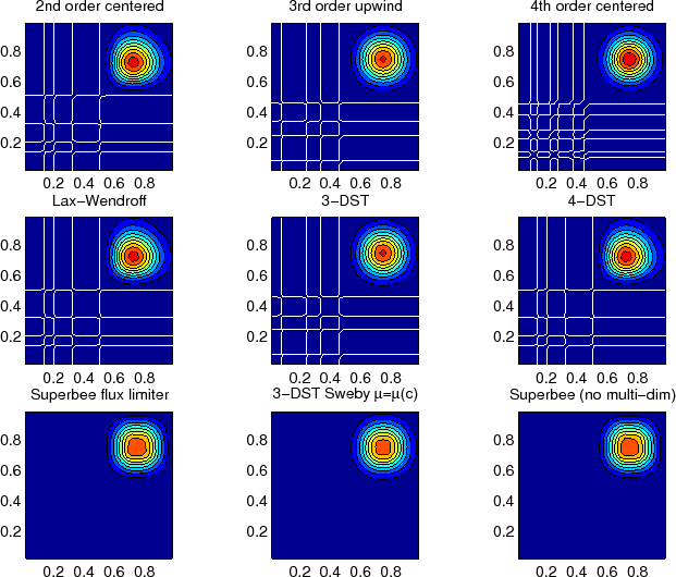
Figure 2.15:
Comparison of advection schemes in two dimensions; diagonal advection
of a resolved Gaussian feature. Courant number is 0.01 with
30 30 points and solutions are shown for T=1/2. White lines
indicate zero crossing (ie. the presence of false minima). The left
column shows the second order schemes; top) centered second order with
Adams-Bashforth, middle) Lax-Wendroff and bottom) Superbee flux
limited. The middle column shows the third order schemes; top) upwind
biased third order with Adams-Bashforth, middle) third order direct
space-time method and bottom) the same with flux limiting. The top
right panel shows the centered fourth order scheme with
Adams-Bashforth and right middle panel shows a fourth order variant on
the DST method. Bottom right panel shows the Superbee flux limiter
(second order) applied independently in each direction (method of
lines).
30 points and solutions are shown for T=1/2. White lines
indicate zero crossing (ie. the presence of false minima). The left
column shows the second order schemes; top) centered second order with
Adams-Bashforth, middle) Lax-Wendroff and bottom) Superbee flux
limited. The middle column shows the third order schemes; top) upwind
biased third order with Adams-Bashforth, middle) third order direct
space-time method and bottom) the same with flux limiting. The top
right panel shows the centered fourth order scheme with
Adams-Bashforth and right middle panel shows a fourth order variant on
the DST method. Bottom right panel shows the Superbee flux limiter
(second order) applied independently in each direction (method of
lines).
|
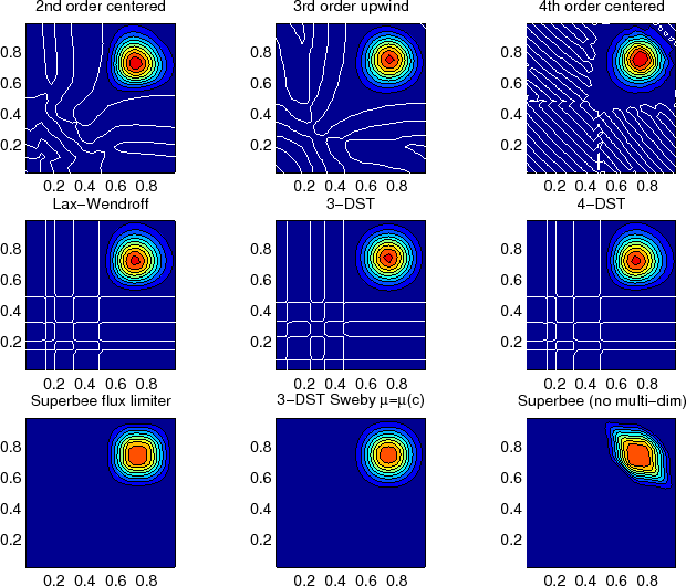
Figure 2.16:
Comparison of advection schemes in two dimensions; diagonal advection
of a resolved Gaussian feature. Courant number is 0.27 with
30
30 points and solutions are shown for T=1/2. White lines
indicate zero crossing (ie. the presence of false minima). The left
column shows the second order schemes; top) centered second order with
Adams-Bashforth, middle) Lax-Wendroff and bottom) Superbee flux
limited. The middle column shows the third order schemes; top) upwind
biased third order with Adams-Bashforth, middle) third order direct
space-time method and bottom) the same with flux limiting. The top
right panel shows the centered fourth order scheme with
Adams-Bashforth and right middle panel shows a fourth order variant on
the DST method. Bottom right panel shows the Superbee flux limiter
(second order) applied independently in each direction (method of
lines).
|
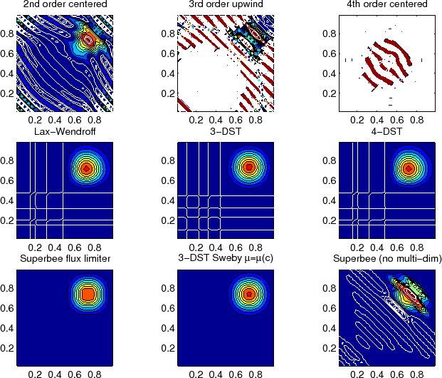
Figure 2.17:
Comparison of advection schemes in two dimensions; diagonal advection
of a resolved Gaussian feature. Courant number is 0.47 with
30
30 points and solutions are shown for T=1/2. White lines
indicate zero crossings and initial maximum values (ie. the presence
of false extrema). The left column shows the second order schemes;
top) centered second order with Adams-Bashforth, middle) Lax-Wendroff
and bottom) Superbee flux limited. The middle column shows the third
order schemes; top) upwind biased third order with Adams-Bashforth,
middle) third order direct space-time method and bottom) the same with
flux limiting. The top right panel shows the centered fourth order
scheme with Adams-Bashforth and right middle panel shows a fourth
order variant on the DST method. Bottom right panel shows the Superbee
flux limiter (second order) applied independently in each direction
(method of lines).
|
In many of the aforementioned advection schemes the behavior in
multiple dimensions is not necessarily as good as the one dimensional
behavior. For instance, a shape preserving monotonic scheme in one
dimension can have severe shape distortion in two dimensions if the
two components of horizontal fluxes are treated independently. There
is a large body of literature on the subject dealing with this problem
and among the fixes are operator and flux splitting methods, corner
flux methods and more. We have adopted a variant on the standard
splitting methods that allows the flux calculations to be implemented
as if in one dimension:
In order to incorporate this method into the general model algorithm,
we compute the effective tendency rather than update the tracer so
that other terms such as diffusion are using the  time-level and
not the updated
time-level and
not the updated  quantities:
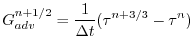 |
(2.204) |
So that the over all time-stepping looks likes:
 |
(2.205) |
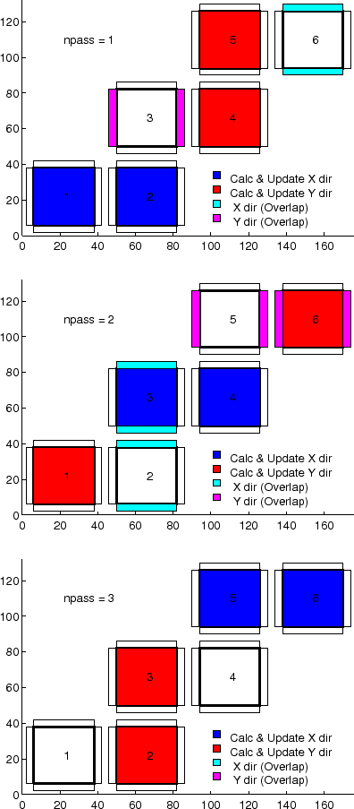
Figure 2.18:
Muti-dimensional advection time-stepping with Cubed-Sphere topology
|
Next: 2.19 Comparison of advection
Up: 2.18 Non-linear advection schemes
Previous: 2.18.3 Third order direct
Contents
mitgcm-support@mitgcm.org
| Copyright © 2006
Massachusetts Institute of Technology |
Last update 2018-01-23 |
 |
|


