|
|
|
|


Next: 2.4 Explicit time-stepping: Adams-Bashforth
Up: 2. Discretization and Algorithm
Previous: 2.2 Pressure method with
Contents
2.3 Pressure method with implicit linear free-surface
The rigid-lid approximation filters out external gravity waves
subsequently modifying the dispersion relation of barotropic Rossby
waves. The discrete form of the elliptic equation has some zero
eigen-values which makes it a potentially tricky or inefficient
problem to solve.
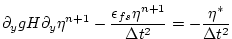
The rigid-lid approximation can be easily replaced by a linearization
of the free-surface equation which can be written:
 |
(2.15) |
which differs from the depth integrated continuity equation with
rigid-lid (2.4) by the time-dependent term
and fresh-water source term.
Equation 2.7 in the rigid-lid
pressure method is then replaced by the time discretization of
2.15 which is:
 |
(2.16) |
where the use of flow at time level  makes the method implicit
and backward in time. The is the preferred scheme since it still
filters the fast unresolved wave motions by damping them. A centered
scheme, such as Crank-Nicholson, would alias the energy of the fast
modes onto slower modes of motion. makes the method implicit
and backward in time. The is the preferred scheme since it still
filters the fast unresolved wave motions by damping them. A centered
scheme, such as Crank-Nicholson, would alias the energy of the fast
modes onto slower modes of motion.
As for the rigid-lid pressure method, equations
2.5, 2.6 and
2.16 can be re-arranged as follows:
 |
 |
 |
(2.17) |
 |
|
 |
(2.18) |
 |
|
 |
(2.19) |
 |
 |
 |
(2.20) |
 |
|
 |
(2.21) |
 |
|
 |
(2.22) |
Equations 2.17
to 2.22, solved sequentially, represent
the pressure method algorithm with a backward implicit, linearized
free surface. The method is still formerly a pressure method because
in the limit of large  the rigid-lid method is
recovered. However, the implicit treatment of the free-surface allows
the flow to be divergent and for the surface pressure/elevation to
respond on a finite time-scale (as opposed to instantly). To recover
the rigid-lid formulation, we introduced a switch-like parameter, the rigid-lid method is
recovered. However, the implicit treatment of the free-surface allows
the flow to be divergent and for the surface pressure/elevation to
respond on a finite time-scale (as opposed to instantly). To recover
the rigid-lid formulation, we introduced a switch-like parameter,
 , which selects between the free-surface and rigid-lid; , which selects between the free-surface and rigid-lid;
 allows the free-surface to evolve; allows the free-surface to evolve;
 imposes the rigid-lid. The evolution in time and location of variables
is exactly as it was for the rigid-lid model so that
Fig. 2.1 is still
applicable. Similarly, the calling sequence, given in
Fig. 2.2, is as for the
pressure-method.
imposes the rigid-lid. The evolution in time and location of variables
is exactly as it was for the rigid-lid model so that
Fig. 2.1 is still
applicable. Similarly, the calling sequence, given in
Fig. 2.2, is as for the
pressure-method.
Next: 2.4 Explicit time-stepping: Adams-Bashforth
Up: 2. Discretization and Algorithm
Previous: 2.2 Pressure method with
Contents
mitgcm-support@dev.mitgcm.org
| Copyright © 2002
Massachusetts Institute of Technology |
 |
|