Home Contact Us Site Map  
 
       
    next up previous contents
Next: 2.3 Pressure method with Up: 2. Discretization and Algorithm Previous: 2.1 Time-stepping   Contents


2.2 Pressure method with rigid-lid

Figure 2.1: A schematic of the evolution in time of the pressure method algorithm. A prediction for the flow variables at time level $ n+1$ is made based only on the explicit terms, $ G^{(n+^1/_2)}$, and denoted $ u^*$, $ v^*$. Next, a pressure field is found such that $ u^{n+1}$, $ v^{n+1}$ will be non-divergent. Conceptually, the $ *$ quantities exist at time level $ n+1$ but they are intermediate and only temporary.
\resizebox{4.0in}{!}{\includegraphics{part2/pressure-method-rigid-lid.eps}}

Figure: Calling tree for the pressure method algorithm (FORWARD_STEP)
% latex2html id marker 4356
\fbox{ \begin{minipage}{4.5in} \begin{tabbing}
aaa ...
...(\ref{eq:un+1-rigid-lid},\ref{eq:vn+1-rigid-lid})
\end{tabbing} \end{minipage} }

The horizontal momentum and continuity equations for the ocean (1.99 and 1.101), or for the atmosphere (1.45 and 1.47), can be summarized by:

$\displaystyle \partial_t u + g \partial_x \eta$ $\displaystyle =$ $\displaystyle G_u$ (2.1)
$\displaystyle \partial_t v + g \partial_y \eta$ $\displaystyle =$ $\displaystyle G_v$ (2.2)
$\displaystyle \partial_x u + \partial_y v + \partial_z w$ $\displaystyle =$ 0 (2.3)

where we are adopting the oceanic notation for brevity. All terms in the momentum equations, except for surface pressure gradient, are encapsulated in the $ G$ vector. The continuity equation, when integrated over the fluid depth, $ H$, and with the rigid-lid/no normal flow boundary conditions applied, becomes:

$\displaystyle \partial_x H \widehat{u} + \partial_y H \widehat{v} = 0$ (2.4)

Here, $ H\widehat{u} = \int_H u dz$ is the depth integral of $ u$, similarly for $ H\widehat{v}$. The rigid-lid approximation sets $ w=0$ at the lid so that it does not move but allows a pressure to be exerted on the fluid by the lid. The horizontal momentum equations and vertically integrated continuity equation are be discretized in time and space as follows:
$\displaystyle u^{n+1} + \Delta t g \partial_x \eta^{n+1}$ $\displaystyle =$ $\displaystyle u^{n} + \Delta t G_u^{(n+1/2)}$ (2.5)
$\displaystyle v^{n+1} + \Delta t g \partial_y \eta^{n+1}$ $\displaystyle =$ $\displaystyle v^{n} + \Delta t G_v^{(n+1/2)}$ (2.6)
$\displaystyle \partial_x H \widehat{u^{n+1}}
+ \partial_y H \widehat{v^{n+1}}$ $\displaystyle =$ 0 (2.7)

As written here, terms on the LHS all involve time level $ n+1$ and are referred to as implicit; the implicit backward time stepping scheme is being used. All other terms in the RHS are explicit in time. The thermodynamic quantities are integrated forward in time in parallel with the flow and will be discussed later. For the purposes of describing the pressure method it suffices to say that the hydrostatic pressure gradient is explicit and so can be included in the vector $ G$.

Substituting the two momentum equations into the depth integrated continuity equation eliminates $ u^{n+1}$ and $ v^{n+1}$ yielding an elliptic equation for $ \eta^{n+1}$. Equations 2.5, 2.6 and 2.7 can then be re-arranged as follows:

$\displaystyle u^{*}$ $\displaystyle =$ $\displaystyle u^{n} + \Delta t G_u^{(n+1/2)}$ (2.8)
$\displaystyle v^{*}$ $\displaystyle =$ $\displaystyle v^{n} + \Delta t G_v^{(n+1/2)}$ (2.9)
$\displaystyle \partial_x \Delta t g H \partial_x \eta^{n+1}
+ \partial_y \Delta t g H \partial_y \eta^{n+1}$ $\displaystyle =$ $\displaystyle \partial_x H \widehat{u^{*}}
+ \partial_y H \widehat{v^{*}}$ (2.10)
$\displaystyle u^{n+1}$ $\displaystyle =$ $\displaystyle u^{*} - \Delta t g \partial_x \eta^{n+1}$ (2.11)
$\displaystyle v^{n+1}$ $\displaystyle =$ $\displaystyle v^{*} - \Delta t g \partial_y \eta^{n+1}$ (2.12)

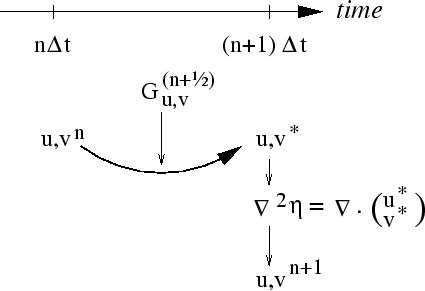
Equations 2.8 to 2.12, solved sequentially, represent the pressure method algorithm used in the model. The essence of the pressure method lies in the fact that any explicit prediction for the flow would lead to a divergence flow field so a pressure field must be found that keeps the flow non-divergent over each step of the integration. The particular location in time of the pressure field is somewhat ambiguous; in Fig. 2.1 we depicted as co-located with the future flow field (time level $ n+1$) but it could equally have been drawn as staggered in time with the flow.

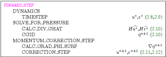
The correspondence to the code is as follows:

  • the prognostic phase, equations 2.8 and 2.9, stepping forward $ u^n$ and $ v^n$ to $ u^{*}$ and $ v^{*}$ is coded in TIMESTEP()
  • the vertical integration, $ H \widehat{u^*}$ and $ H
\widehat{v^*}$, divergence and inversion of the elliptic operator in equation 2.10 is coded in SOLVE_FOR_PRESSURE()
  • finally, the new flow field at time level $ n+1$ given by equations 2.11 and 2.12 is calculated in CORRECTION_STEP().
The calling tree for these routines is given in Fig. 2.2.

2.2.0.0.1 Need to discuss implicit viscosity somewhere:


$\displaystyle \frac{1}{\Delta t} u^{n+1} - \partial_z A_v \partial_z u^{n+1}
+ g \partial_x \eta^{n+1}$ $\displaystyle =$ $\displaystyle \frac{1}{\Delta t} u^{n} +
G_u^{(n+1/2)}$ (2.13)
$\displaystyle \frac{1}{\Delta t} v^{n+1} - \partial_z A_v \partial_z v^{n+1}
+ g \partial_y \eta^{n+1}$ $\displaystyle =$ $\displaystyle \frac{1}{\Delta t} v^{n} + G_v^{(n+1/2)}$ (2.14)


next up previous contents
Next: 2.3 Pressure method with Up: 2. Discretization and Algorithm Previous: 2.1 Time-stepping   Contents
mitgcm-support@dev.mitgcm.org
Copyright © 2002 Massachusetts Institute of Technology