|
|
|
|


Next: 2.7 Staggered baroclinic time-stepping
Up: 2. Discretization and Algorithm
Previous: 2.5 Implicit time-stepping: backward
Contents
2.6 Synchronous time-stepping: variables co-located in time
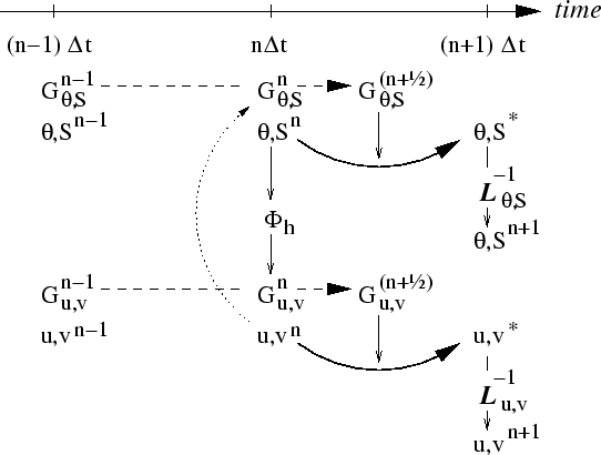
Figure 2.4:
A schematic of the explicit Adams-Bashforth and implicit time-stepping
phases of the algorithm. All prognostic variables are co-located in
time. Explicit tendencies are evaluated at time level  as a
function of the state at that time level (dotted arrow). The explicit
tendency from the previous time level, as a
function of the state at that time level (dotted arrow). The explicit
tendency from the previous time level,  , is used to extrapolate
tendencies to , is used to extrapolate
tendencies to  (dashed arrow). This extrapolated tendency
allows variables to be stably integrated forward-in-time to render an
estimate ( (dashed arrow). This extrapolated tendency
allows variables to be stably integrated forward-in-time to render an
estimate ( -variables) at the -variables) at the  time level (solid
arc-arrow). The operator time level (solid
arc-arrow). The operator  formed from implicit-in-time terms
is solved to yield the state variables at time level . formed from implicit-in-time terms
is solved to yield the state variables at time level .
|
|
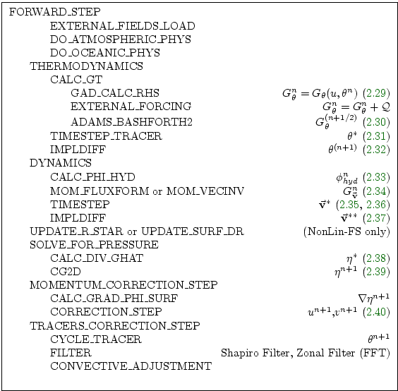
Figure 2.5:
Calling tree for the overall synchronous algorithm using
Adams-Bashforth time-stepping.
The place where the model geometry
(hFac factors) is updated is added here but is only relevant
for the non-linear free-surface algorithm.
For completeness, the external forcing,
ocean and atmospheric physics have been added, although they are mainly
optional
|
|
The Adams-Bashforth extrapolation of explicit tendencies fits neatly
into the pressure method algorithm when all state variables are
co-located in time. Fig. 2.4 illustrates
the location of variables in time and the evolution of the algorithm
with time. The algorithm can be represented by the sequential solution
of the follow equations:
 |
 |
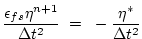
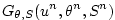 |
(2.29) |
 |
|
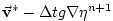
 |
(2.30) |
 |
|
 |
(2.31) |
 |
|
 |
(2.32) |
 |
|
 |
(2.33) |
 |
|
 |
(2.34) |
 |
|
 |
(2.35) |
 |
|
 |
(2.36) |
 |
|
 |
(2.37) |
 |
|
 |
(2.38) |
 |
 |
 |
(2.39) |
 |
|
 |
(2.40) |
Fig. 2.4 illustrates the location of
variables in time and evolution of the algorithm with time. The
Adams-Bashforth extrapolation of the tracer tendencies is illustrated
by the dashed arrow, the prediction at is indicated by the
solid arc. Inversion of the implicit terms,
 , then yields the new tracer fields at . All
these operations are carried out in subroutine THERMODYNAMICS an
subsidiaries, which correspond to equations 2.29 to
2.32.
Similarly illustrated is the Adams-Bashforth extrapolation of
accelerations, stepping forward and solving of implicit viscosity and
surface pressure gradient terms, corresponding to equations
2.34 to 2.40.
These operations are carried out in subroutines DYNAMCIS, SOLVE_FOR_PRESSURE and MOMENTUM_CORRECTION_STEP. This, then,
represents an entire algorithm for stepping forward the model one
time-step. The corresponding calling tree is given in
2.5. , then yields the new tracer fields at . All
these operations are carried out in subroutine THERMODYNAMICS an
subsidiaries, which correspond to equations 2.29 to
2.32.
Similarly illustrated is the Adams-Bashforth extrapolation of
accelerations, stepping forward and solving of implicit viscosity and
surface pressure gradient terms, corresponding to equations
2.34 to 2.40.
These operations are carried out in subroutines DYNAMCIS, SOLVE_FOR_PRESSURE and MOMENTUM_CORRECTION_STEP. This, then,
represents an entire algorithm for stepping forward the model one
time-step. The corresponding calling tree is given in
2.5.
Next: 2.7 Staggered baroclinic time-stepping
Up: 2. Discretization and Algorithm
Previous: 2.5 Implicit time-stepping: backward
Contents
mitgcm-support@dev.mitgcm.org
| Copyright © 2002
Massachusetts Institute of Technology |
 |
|