Home Contact Us Site Map  
 
       
    next up previous contents
Next: 2.8 Non-hydrostatic formulation Up: 2. Discretization and Algorithm Previous: 2.6 Synchronous time-stepping: variables   Contents


2.7 Staggered baroclinic time-stepping

Figure 2.6: A schematic of the explicit Adams-Bashforth and implicit time-stepping phases of the algorithm but with staggering in time of thermodynamic variables with the flow. Explicit momentum tendencies are evaluated at time level $ n-1/2$ as a function of the flow field at that time level $ n-1/2$. The explicit tendency from the previous time level, $ n-3/2$, is used to extrapolate tendencies to $ n$ (dashed arrow). The hydrostatic pressure/geo-potential $ \phi _{hyd}$ is evaluated directly at time level $ n$ (vertical arrows) and used with the extrapolated tendencies to step forward the flow variables from $ n-1/2$ to $ n+1/2$ (solid arc-arrow). The implicit-in-time operator $ {\cal L}_{\bf u,v}$ (vertical arrows) is then applied to the previous estimation of the the flow field ($ *$-variables) and yields to the two velocity components $ u,v$ at time level $ n+1/2$. These are then used to calculate the advection term (dashed arc-arrow) of the thermo-dynamics tendencies at time step $ n$. The extrapolated thermodynamics tendency, from time level $ n-1$ and $ n$ to $ n+1/2$, allows thermodynamic variables to be stably integrated forward-in-time (solid arc-arrow) up to time level $ n+1$.
\resizebox{5.5in}{!}{\includegraphics{part2/adams-bashforth-staggered.eps}}

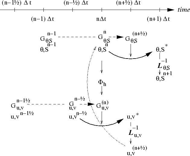
For well stratified problems, internal gravity waves may be the limiting process for determining a stable time-step. In the circumstance, it is more efficient to stagger in time the thermodynamic variables with the flow variables. Fig. 2.6 illustrates the staggering and algorithm. The key difference between this and Fig. 2.4 is that the thermodynamic variables are solved after the dynamics, using the recently updated flow field. This essentially allows the gravity wave terms to leap-frog in time giving second order accuracy and more stability.

The essential change in the staggered algorithm is that the thermodynamics solver is delayed from half a time step, allowing the use of the most recent velocities to compute the advection terms. Once the thermodynamics fields are updated, the hydrostatic pressure is computed to step forwrad the dynamics. Note that the pressure gradient must also be taken out of the Adams-Bashforth extrapolation. Also, retaining the integer time-levels, $ n$ and $ n+1$, does not give a user the sense of where variables are located in time. Instead, we re-write the entire algorithm, 2.29 to 2.40, annotating the position in time of variables appropriately:

$\displaystyle \phi^{n}_{hyd}$ $\displaystyle =$ $\displaystyle \int b(\theta^{n},S^{n}) dr$ (2.41)
$\displaystyle \vec{\bf G}_{\vec{\bf v}}^{n-1/2}$ $\displaystyle =$ $\displaystyle \vec{\bf G}_{\vec{\bf v}} ( \vec{\bf v}^{n-1/2} )$ (2.42)
$\displaystyle \vec{\bf G}_{\vec{\bf v}}^{(n)}$ $\displaystyle =$ $\displaystyle (3/2 + \epsilon_{AB} ) \vec{\bf G}_{\vec{\bf v}}^{n-1/2} - (1/2 + \epsilon_{AB} ) \vec{\bf G}_{\vec{\bf v}}^{n-3/2}$ (2.43)
$\displaystyle \vec{\bf v}^{*}$ $\displaystyle =$ $\displaystyle \vec{\bf v}^{n-1/2} + \Delta t \left( \vec{\bf G}_{\vec{\bf v}}^{(n)} - \nabla \phi_{hyd}^{n} \right)$ (2.44)
$\displaystyle \vec{\bf v}^{**}$ $\displaystyle =$ $\displaystyle {\cal L}_{\vec{\bf v}}^{-1} ( \vec{\bf v}^* )$ (2.45)
$\displaystyle \eta^*$ $\displaystyle =$ $\displaystyle \epsilon_{fs} \left( \eta^{n-1/2} + \Delta t (P-E)^n \right)- \Delta t
\nabla \cdot H \widehat{ \vec{\bf v}^{**} }$ (2.46)
$\displaystyle \nabla \cdot g H \nabla \eta^{n+1/2}$ $\displaystyle -$ $\displaystyle \frac{\epsilon_{fs} \eta^{n+1/2}}{\Delta t^2}
~ = ~ - \frac{\eta^*}{\Delta t^2}$ (2.47)
$\displaystyle \vec{\bf v}^{n+1/2}$ $\displaystyle =$ $\displaystyle \vec{\bf v}^{*} - \Delta t g \nabla \eta^{n+1/2}$ (2.48)
$\displaystyle G_{\theta,S}^{n}$ $\displaystyle =$ $\displaystyle G_{\theta,S} ( u^{n+1/2}, \theta^{n}, S^{n} )$ (2.49)
$\displaystyle G_{\theta,S}^{(n+1/2)}$ $\displaystyle =$ $\displaystyle (3/2+\epsilon_{AB}) G_{\theta,S}^{n}-(1/2+\epsilon_{AB}) G_{\theta,S}^{n-1}$ (2.50)
$\displaystyle (\theta^*,S^*)$ $\displaystyle =$ $\displaystyle (\theta^{n},S^{n}) + \Delta t G_{\theta,S}^{(n+1/2)}$ (2.51)
$\displaystyle (\theta^{n+1},S^{n+1})$ $\displaystyle =$ $\displaystyle {\cal L}^{-1}_{\theta,S} (\theta^*,S^*)$ (2.52)

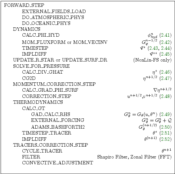
The corresponding calling tree is given in 2.7. The staggered algorithm is activated with the run-time flag staggerTimeStep=.TRUE. in parameter file data, namelist PARM01.

Figure 2.7: Calling tree for the overall staggered algorithm using Adams-Bashforth time-stepping. The place where the model geometry (hFac factors) is updated is added here but is only relevant for the non-linear free-surface algorithm.
% latex2html id marker 4550
\fbox{ \begin{minipage}{4.7in} \begin{tabbing}
aaa ...
...lter (FFT) \\
\>\> CONVECTIVE\_ADJUSTMENT \\lq  \\
\end{tabbing} \end{minipage} }

The only difficulty with this approach is apparent in equation 2.49 and illustrated by the dotted arrow connecting $ u,v^{n+1/2}$ with $ G_\theta^{n}$. The flow used to advect tracers around is not naturally located in time. This could be avoided by applying the Adams-Bashforth extrapolation to the tracer field itself and advecting that around but this approach is not yet available. We're not aware of any detrimental effect of this feature. The difficulty lies mainly in interpretation of what time-level variables and terms correspond to.


next up previous contents
Next: 2.8 Non-hydrostatic formulation Up: 2. Discretization and Algorithm Previous: 2.6 Synchronous time-stepping: variables   Contents
mitgcm-support@dev.mitgcm.org
Copyright © 2002 Massachusetts Institute of Technology