|
|
|
|


Next: 3.10.2 Equations solved
Up: 3.10 Baroclinic Gyre MITgcm
Previous: 3.10 Baroclinic Gyre MITgcm
Contents
This example experiment demonstrates using the MITgcm to simulate
a baroclinic, wind-forced, ocean gyre circulation. The experiment
is a numerical rendition of the gyre circulation problem similar
to the problems described analytically by Stommel in 1966
Stommel [1948] and numerically in Holland et. al Holland and Lin [975a].
In this experiment the model is configured to represent a mid-latitude
enclosed sector of fluid on a sphere,
 in
lateral extent. The fluid is
in
lateral extent. The fluid is  km deep and is forced
by a constant in time zonal wind stress,
km deep and is forced
by a constant in time zonal wind stress,
 , that varies
sinusoidally in the north-south direction. Topologically the simulated
domain is a sector on a sphere and the coriolis parameter,
, that varies
sinusoidally in the north-south direction. Topologically the simulated
domain is a sector on a sphere and the coriolis parameter,  , is defined
according to latitude,
, is defined
according to latitude, 
 |
(3.10) |
with the rotation rate,  set to
 .
.
The sinusoidal wind-stress variations are defined according to
 |
(3.11) |
where
 is the lateral domain extent (
 ) and
) and
 is set to
 .
.
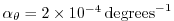
Figure 3.2
summarizes the configuration simulated.
In contrast to the example in section 3.9, the
current experiment simulates a spherical polar domain. As indicated
by the axes in the lower left of the figure the model code works internally
in a locally orthogonal coordinate  . For this experiment description
the local orthogonal model coordinate
is synonymous
with the coordinates
. For this experiment description
the local orthogonal model coordinate
is synonymous
with the coordinates
 shown in figure
1.16
shown in figure
1.16
The experiment has four levels in the vertical, each of equal thickness,
 m. Initially the fluid is stratified with a reference
potential temperature profile,
m. Initially the fluid is stratified with a reference
potential temperature profile,
 C,
C,
 C,
C,
 C,
C,
 C. The equation of state used in this experiment is
linear
C. The equation of state used in this experiment is
linear
 |
(3.12) |
which is implemented in the model as a density anomaly equation
 |
(3.13) |
with
 and
and
 . Integrated forward in
this configuration the model state variable theta is equivalent to
either in-situ temperature,
. Integrated forward in
this configuration the model state variable theta is equivalent to
either in-situ temperature,  , or potential temperature,
  . For
consistency with later examples, in which the equation of state is
non-linear, we use
to represent temperature here. This is
the quantity that is carried in the model core equations.
. For
consistency with later examples, in which the equation of state is
non-linear, we use
to represent temperature here. This is
the quantity that is carried in the model core equations.
Figure 3.2:
Schematic of simulation domain and wind-stress forcing function
for the four-layer gyre numerical experiment. The domain is enclosed by solid
walls at  E,
E,
N and
N.
An initial stratification is
imposed by setting the potential temperature,
, in each layer.
The vertical spacing,
E,
E,
N and
N.
An initial stratification is
imposed by setting the potential temperature,
, in each layer.
The vertical spacing,  , is constant and equal to
  m.
m.
 |
Next: 3.10.2 Equations solved
Up: 3.10 Baroclinic Gyre MITgcm
Previous: 3.10 Baroclinic Gyre MITgcm
Contents
mitgcm-support@mitgcm.org
| Copyright © 2006
Massachusetts Institute of Technology |
Last update 2018-01-23 |
 |
|


