|
|
|
|


Next: 3.10.3 Discrete Numerical Configuration
Up: 3.10 Baroclinic Gyre MITgcm
Previous: 3.10.1 Overview
Contents
For this problem
the implicit free surface, HPE (see section 1.3.4.2) form of the
equations described in Marshall et. al Marshall et al. [1997b] are
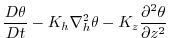
employed. The flow is three-dimensional with just temperature,  , as
an active tracer. The equation of state is linear.
A horizontal Laplacian operator
, as
an active tracer. The equation of state is linear.
A horizontal Laplacian operator
 provides viscous
dissipation and provides a diffusive sub-grid scale closure for the
temperature equation. A wind-stress momentum forcing is added to the momentum
equation for the zonal flow,
provides viscous
dissipation and provides a diffusive sub-grid scale closure for the
temperature equation. A wind-stress momentum forcing is added to the momentum
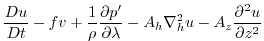
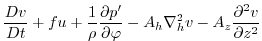
equation for the zonal flow,  . Other terms in the model
are explicitly switched off for this experiment configuration (see section
3.10.4 ). This yields an active set of equations
solved in this configuration, written in spherical polar coordinates as
follows
. Other terms in the model
are explicitly switched off for this experiment configuration (see section
3.10.4 ). This yields an active set of equations
solved in this configuration, written in spherical polar coordinates as
follows
 |
 |
 |
(3.14) |
 |
|
0 |
(3.15) |
 |
|
0 |
(3.16) |
 |
|
0 |
(3.17) |
 |
|
 |
(3.18) |
 |
|
 |
(3.19) |
 |
|
 |
(3.20) |
 |
|
0 |
(3.21) |
where
and  are the components of the horizontal
flow vector
are the components of the horizontal
flow vector  on the sphere (
 ).
The terms
).
The terms
 and
and
 are the components of the vertical
integral term given in equation 1.35 and
explained in more detail in section 2.4.
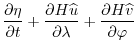
However, for the problem presented here, the continuity relation (equation
3.16) differs from the general form given
in section 2.4,
equation 2.15, because the source terms
are the components of the vertical
integral term given in equation 1.35 and
explained in more detail in section 2.4.
However, for the problem presented here, the continuity relation (equation
3.16) differs from the general form given
in section 2.4,
equation 2.15, because the source terms
 are all 0
.
are all 0
.
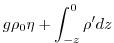
The pressure field,
 , is separated into a barotropic part
due to variations in sea-surface height,
, is separated into a barotropic part
due to variations in sea-surface height,  , and a hydrostatic
part due to variations in density,
, and a hydrostatic
part due to variations in density,
 , integrated
through the water column.
, integrated
through the water column.
The suffices  indicate surface layer and the interior of the domain.
The windstress forcing,
indicate surface layer and the interior of the domain.
The windstress forcing,
 , is applied in the surface layer
by a source term in the zonal momentum equation. In the ocean interior
this term is zero.
, is applied in the surface layer
by a source term in the zonal momentum equation. In the ocean interior
this term is zero.
In the momentum equations
lateral and vertical boundary conditions for the
 and
and
 operators are specified
when the numerical simulation is run - see section
3.10.4. For temperature
the boundary condition is ``zero-flux''
e.g.
operators are specified
when the numerical simulation is run - see section
3.10.4. For temperature
the boundary condition is ``zero-flux''
e.g.
 .
.
Next: 3.10.3 Discrete Numerical Configuration
Up: 3.10 Baroclinic Gyre MITgcm
Previous: 3.10.1 Overview
Contents
mitgcm-support@mitgcm.org
| Copyright © 2006
Massachusetts Institute of Technology |
Last update 2018-01-23 |
 |
|


