


Next: 3.10.4 Code Configuration
Up: 3.10 Baroclinic Gyre MITgcm
Previous: 3.10.2 Equations solved
Contents
Subsections
The domain is discretised with
a uniform grid spacing in latitude and longitude
 , so
that there are sixty grid cells in the zonal and meridional directions.
Vertically the
model is configured with four layers with constant depth,
, so
that there are sixty grid cells in the zonal and meridional directions.
Vertically the
model is configured with four layers with constant depth,
 , of
, of  m. The internal, locally orthogonal, model coordinate
variables
m. The internal, locally orthogonal, model coordinate
variables  and
and  are initialized from the values of
 ,
,  ,
,
 and
and
 in
radians according to
in
radians according to
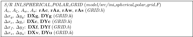
The procedure for generating a set of internal grid variables from a
spherical polar grid specification is discussed in section
2.11.4.
As described in 2.16, the time evolution of potential
temperature,
 , (equation 3.17)
is evaluated prognostically. The centered second-order scheme with
Adams-Bashforth time stepping described in section
2.16.1 is used to step forward the temperature
equation. Prognostic terms in
the momentum equations are solved using flux form as
described in section 2.14.
The pressure forces that drive the fluid motions, (
, (equation 3.17)
is evaluated prognostically. The centered second-order scheme with
Adams-Bashforth time stepping described in section
2.16.1 is used to step forward the temperature
equation. Prognostic terms in
the momentum equations are solved using flux form as
described in section 2.14.
The pressure forces that drive the fluid motions, (
 and
and
 ), are found by summing pressure due to surface
elevation
), are found by summing pressure due to surface
elevation  and the hydrostatic pressure. The hydrostatic part of the
pressure is diagnosed explicitly by integrating density. The sea-surface
height,
, is diagnosed using an implicit scheme. The pressure
field solution method is described in sections
2.4 and
1.3.6.
and the hydrostatic pressure. The hydrostatic part of the
pressure is diagnosed explicitly by integrating density. The sea-surface
height,
, is diagnosed using an implicit scheme. The pressure
field solution method is described in sections
2.4 and
1.3.6.
The Laplacian viscosity coefficient,  , is set to
 .
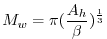
This value is chosen to yield a Munk layer width,
.
This value is chosen to yield a Munk layer width,
 |
|
|
(3.24) |
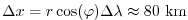
of
 km. This is greater than the model
resolution in mid-latitudes
km. This is greater than the model
resolution in mid-latitudes
 at
at
 , ensuring that the frictional
boundary layer is well resolved.
, ensuring that the frictional
boundary layer is well resolved.
The model is stepped forward with a
time step
 secs. With this time step the stability
parameter to the horizontal Laplacian friction
secs. With this time step the stability
parameter to the horizontal Laplacian friction
 |
|
|
(3.25) |
evaluates to 0.012, which is well below the 0.3 upper limit
for stability for this term under ABII time-stepping.
The vertical dissipation coefficient,  , is set to
 . The associated stability limit
 |
|
|
(3.26) |
evaluates to
 which is again well below
the upper limit.
The values of
and
are also used for the horizontal (
which is again well below
the upper limit.
The values of
and
are also used for the horizontal ( )
and vertical (
)
and vertical ( ) diffusion coefficients for temperature respectively.
The numerical stability for inertial oscillations
 |
|
|
(3.27) |
evaluates to  , which is well below the
  upper
limit for stability.
upper
limit for stability.
The advective CFL for a extreme maximum
horizontal flow
speed of

 |
|
|
(3.28) |
evaluates to
 . This is well below the stability
limit of 0.5.
. This is well below the stability
limit of 0.5.
The stability parameter for internal gravity waves
propagating at

 |
|
|
(3.29) |
evaluates to
 . This is well below the linear
stability limit of 0.25.
. This is well below the linear
stability limit of 0.25.
Next: 3.10.4 Code Configuration
Up: 3.10 Baroclinic Gyre MITgcm
Previous: 3.10.2 Equations solved
Contents
mitgcm-support@mitgcm.org
| Copyright © 2006
Massachusetts Institute of Technology |
Last update 2018-01-23 |
 |
|


