


Next: 3.12.3 Experiment Configuration
Up: 3.12 Global Ocean MITgcm
Previous: 3.12.1 Overview
Contents
Subsections
The model is configured in hydrostatic form. The domain is
discretised with a uniform grid spacing in latitude and longitude on
the sphere
 , so that there are
ninety grid cells in the zonal and forty in the meridional
direction. The internal model coordinate variables
, so that there are
ninety grid cells in the zonal and forty in the meridional
direction. The internal model coordinate variables  and
and  are
initialized according to
are
initialized according to
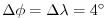
Arctic polar regions are not
included in this experiment. Meridionally the model extends from
 to
to
 .
Vertically the model is configured with fifteen layers with the
following thicknesses:
.
Vertically the model is configured with fifteen layers with the
following thicknesses:


(here the numeric subscript indicates the model level index number,  ) to
give a total depth,
) to
give a total depth,  , of
, of
 .
The implicit free surface form of the pressure equation described in
Marshall et al. [1997b] is employed. A Laplacian operator,
.
The implicit free surface form of the pressure equation described in
Marshall et al. [1997b] is employed. A Laplacian operator,  , provides viscous
dissipation. Thermal and haline diffusion is also represented by a Laplacian operator.
, provides viscous
dissipation. Thermal and haline diffusion is also represented by a Laplacian operator.
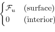
Wind-stress forcing is added to the momentum equations in (3.37)
for both the zonal flow,  and the meridional flow
  , according to equations
(3.31) and (3.32).
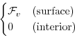
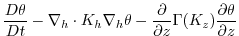
Thermodynamic forcing inputs are added to the equations
in (3.37) for
potential temperature,
, according to equations
(3.31) and (3.32).
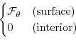
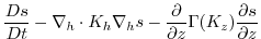
Thermodynamic forcing inputs are added to the equations
in (3.37) for
potential temperature,  , and salinity,
  , according to equations
(3.33) and (3.34).
This produces a set of equations solved in this configuration as follows:
, according to equations
(3.33) and (3.34).
This produces a set of equations solved in this configuration as follows:
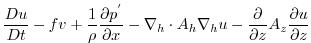 |
 |
 |
(3.37) |
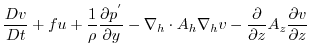 |
|
 |
(3.38) |
 |
|
0 |
(3.39) |
 |
|
 |
(3.40) |
 |
|
 |
(3.41) |
 |
|
 |
(3.42) |
where
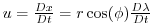 and
and
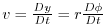 are the zonal and meridional components of the
flow vector,
are the zonal and meridional components of the
flow vector,  , on the sphere. As described in
MITgcm Numerical Solution Procedure 2, the time
evolution of potential temperature,
, equation is solved prognostically.
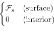
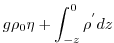
The total pressure,
, on the sphere. As described in
MITgcm Numerical Solution Procedure 2, the time
evolution of potential temperature,
, equation is solved prognostically.
The total pressure,  , is diagnosed by summing pressure due to surface
elevation
, is diagnosed by summing pressure due to surface
elevation  and the hydrostatic pressure.
The Laplacian dissipation coefficient,  , is set to
 .
This value is chosen to yield a Munk layer width [Adcroft, 1995],
.
This value is chosen to yield a Munk layer width [Adcroft, 1995],
| |
|
 |
(3.43) |
of
 km. This is greater than the model
resolution in low-latitudes,
km. This is greater than the model
resolution in low-latitudes,
 , ensuring that the frictional
boundary layer is adequately resolved.
, ensuring that the frictional
boundary layer is adequately resolved.
The model is stepped forward with a time step
 for thermodynamic variables and
 for momentum terms. With this time step,
the stability parameter to the horizontal Laplacian friction
[Adcroft, 1995]
for momentum terms. With this time step,
the stability parameter to the horizontal Laplacian friction
[Adcroft, 1995]
| |
|
 |
(3.44) |
evaluates to 0.6 at a latitude of
 , which
is above the 0.3 upper limit for stability, but the zonal grid spacing
, which
is above the 0.3 upper limit for stability, but the zonal grid spacing
 is smallest at
where
is smallest at
where
 and the stability
criterion is already met 1 grid cell equatorwards (at
and the stability
criterion is already met 1 grid cell equatorwards (at
 ).
).
The vertical dissipation coefficient,  , is set to
 . The associated stability limit
| |
|
 |
(3.45) |
evaluates to  for the smallest model
level spacing (
for the smallest model
level spacing (
 ) which is well below
the upper stability limit.
) which is well below
the upper stability limit.
The numerical stability for inertial oscillations
[Adcroft, 1995]
| |
|
 |
(3.46) |
evaluates to  for
for
 , which is
below the
, which is
below the  upper limit for stability.
The advective CFL [Adcroft, 1995] for a extreme maximum
horizontal flow
speed of

| |
|
 |
(3.47) |
evaluates to
 . This is well below the stability
limit of 0.5.
. This is well below the stability
limit of 0.5.
The stability parameter for internal gravity waves propagating
with a maximum speed of
 [Adcroft, 1995]
| |
|
 |
(3.48) |
evaluates to
 . This is close to the linear
stability limit of 0.5.
. This is close to the linear
stability limit of 0.5.
Next: 3.12.3 Experiment Configuration
Up: 3.12 Global Ocean MITgcm
Previous: 3.12.1 Overview
Contents
mitgcm-support@mitgcm.org
| Copyright © 2006
Massachusetts Institute of Technology |
Last update 2018-01-23 |
 |
|


