|
|
|
|


Next: 3.15.6 Running the example
Up: 3.15 Surface Driven Convection
Previous: 3.15.4 Numerical stability criteria
Contents
Subsections
The model configuration for this experiment resides under the directory
verification/convection/. The experiment files
- code/CPP_EEOPTIONS.h
- code/CPP_OPTIONS.h,
- code/SIZE.h.
- input/data
- input/data.pkg
- input/eedata,
- input/Qsurf.bin,
contain the code customisations and parameter settings for this
experiment. Below we describe these experiment-specific customisations.
This file uses standard default values and does not contain
customisations for this experiment.
This file uses standard default values and does not contain
customisations for this experiment.
Three lines are customized in this file. These prescribe the domain grid dimensions.
- Line 36,
sNx=64,
this line sets
the lateral domain extent in grid points for the
axis aligned with the  -coordinate.
- Line 37,
sNy=64,
this line sets
the lateral domain extent in grid points for the
axis aligned with the  -coordinate.
- Line 46,
Nr=20,
this line sets
the vertical domain extent in grid points.
C
 C
C  C
C /========================================================== C | SIZE.h Declare size of underlying computational grid. |
C |==========================================================|
C | The design here support a three-dimensional model grid |
C | with indices I,J and K. The three-dimensional domain |
C | is comprised of nPx*nSx blocks of size sNx along one axis|
C | nPy*nSy blocks of size sNy along another axis and one |
C | block of size Nz along the final axis. |
C | Blocks have overlap regions of size OLx and OLy along the|
C | dimensions that are subdivided. |
C =========================================================/
C Voodoo numbers controlling data layout.
C sNx - No. X points in sub-grid.
C sNy - No. Y points in sub-grid.
C OLx - Overlap extent in X.
C OLy - Overlat extent in Y.
C nSx - No. sub-grids in X.
C nSy - No. sub-grids in Y.
C nPx - No. of processes to use in X.
C nPy - No. of processes to use in Y.
C Nx - No. points in X for the total domain.
C Ny - No. points in Y for the total domain.
C Nr - No. points in Z for full process domain.
INTEGER sNx
INTEGER sNy
INTEGER OLx
INTEGER OLy
INTEGER nSx
INTEGER nSy
INTEGER nPx
INTEGER nPy
INTEGER Nx
INTEGER Ny
INTEGER Nr
PARAMETER (
& sNx = 64,
& sNy = 64,
& OLx = 3,
& OLy = 3,
& nSx = 1,
& nSy = 1,
& nPx = 1,
& nPy = 1,
& Nx = sNx*nSx*nPx,
& Ny = sNy*nSy*nPy,
& Nr = 20)
C
C /========================================================== C | SIZE.h Declare size of underlying computational grid. |
C |==========================================================|
C | The design here support a three-dimensional model grid |
C | with indices I,J and K. The three-dimensional domain |
C | is comprised of nPx*nSx blocks of size sNx along one axis|
C | nPy*nSy blocks of size sNy along another axis and one |
C | block of size Nz along the final axis. |
C | Blocks have overlap regions of size OLx and OLy along the|
C | dimensions that are subdivided. |
C =========================================================/
C Voodoo numbers controlling data layout.
C sNx - No. X points in sub-grid.
C sNy - No. Y points in sub-grid.
C OLx - Overlap extent in X.
C OLy - Overlat extent in Y.
C nSx - No. sub-grids in X.
C nSy - No. sub-grids in Y.
C nPx - No. of processes to use in X.
C nPy - No. of processes to use in Y.
C Nx - No. points in X for the total domain.
C Ny - No. points in Y for the total domain.
C Nr - No. points in Z for full process domain.
INTEGER sNx
INTEGER sNy
INTEGER OLx
INTEGER OLy
INTEGER nSx
INTEGER nSy
INTEGER nPx
INTEGER nPy
INTEGER Nx
INTEGER Ny
INTEGER Nr
PARAMETER (
& sNx = 64,
& sNy = 64,
& OLx = 3,
& OLy = 3,
& nSx = 1,
& nSy = 1,
& nPx = 1,
& nPy = 1,
& Nx = sNx*nSx*nPx,
& Ny = sNy*nSy*nPy,
& Nr = 20)
C MAX_OLX - Set to the maximum overlap region size of any array
C MAX_OLY that will be exchanged. Controls the sizing of exch
C routine buufers.
INTEGER MAX_OLX
INTEGER MAX_OLY
PARAMETER ( MAX_OLX = OLx,
& MAX_OLY = OLy )
This file, reproduced completely below, specifies the main parameters
for the experiment. The parameters that are significant for this configuration
are
- Line 4,
4 tRef=20*20.0,
this line sets
the initial and reference values of potential temperature at each model
level in units of
 . Here the value is arbitrary since, in this case, the
flow evolves independently of the absolute magnitude of the reference temperature.
For each depth level the initial and reference profiles will be uniform in
and
. The values specified are read into the
variable
tRef
in the model code, by procedure
S/R INI_PARMS (ini_parms.F)
.
The temperature field is initialised, by procedure
S/R INI_THETA (ini_theta.F)
.
. Here the value is arbitrary since, in this case, the
flow evolves independently of the absolute magnitude of the reference temperature.
For each depth level the initial and reference profiles will be uniform in
and
. The values specified are read into the
variable
tRef
in the model code, by procedure
S/R INI_PARMS (ini_parms.F)
.
The temperature field is initialised, by procedure
S/R INI_THETA (ini_theta.F)
.
- Line 5,
5 sRef=20*35.0,
this line sets the initial and reference values of salinity at each model
level in units of ppt. In this case salinity is set to an (arbitrary) uniform value of
35.0 ppt. However since, in this example, density is independent of salinity,
an appropriatly defined initial salinity could provide a useful passive
tracer. For each depth level the initial and reference profiles will be uniform in
and
. The values specified are read into the
variable
sRef
in the model code, by procedure
S/R INI_PARMS (ini_parms.F)
.
The salinity field is initialised, by procedure
S/R INI_SALT (ini_salt.F)
.
- Line 6,
6 viscAh=0.1,
this line sets the horizontal laplacian dissipation coefficient to
0.1
 . Boundary conditions
for this operator are specified later.
The variable
viscAh
is read in the routine
S/R INI_PARMS (ini_params.F)
and applied in routines
S/R CALC_MOM_RHS (calc_mom_rhs.F)
and
S/R CALC_GW (calc_gw.F)
.
. Boundary conditions
for this operator are specified later.
The variable
viscAh
is read in the routine
S/R INI_PARMS (ini_params.F)
and applied in routines
S/R CALC_MOM_RHS (calc_mom_rhs.F)
and
S/R CALC_GW (calc_gw.F)
.
- Line 7,
7 viscAz=0.1,
this line sets the vertical laplacian frictional dissipation coefficient to
0.1
. Boundary conditions
for this operator are specified later.
The variable
viscAz
is read in the routine
S/R INI_PARMS (ini_parms.F)
and is copied into model general vertical coordinate variable
viscAr
. At each time step, the viscous term contribution to the momentum equations
is calculated in routine
S/R CALC_DIFFUSIVITY (calc_diffusivity.F)
.
- Line 8,
no_slip_sides=.FALSE.
this line selects a free-slip lateral boundary condition for
the horizontal laplacian friction operator
e.g.
 =0 along boundaries in
and
=0 along boundaries in
and
 =0 along boundaries in
.
The variable
no_slip_sides
is read in the routine
S/R INI_PARMS (ini_parms.F)
and the boundary condition is evaluated in routine
S/R CALC_MOM_RHS (calc_mom_rhs.F)
.
=0 along boundaries in
.
The variable
no_slip_sides
is read in the routine
S/R INI_PARMS (ini_parms.F)
and the boundary condition is evaluated in routine
S/R CALC_MOM_RHS (calc_mom_rhs.F)
.
- Lines 9,
no_slip_bottom=.TRUE.
this line selects a no-slip boundary condition for the bottom
boundary condition in the vertical laplacian friction operator
e.g.  at
at  , where
  is the local depth of the domain.
The variable
no_slip_bottom
is read in the routine
S/R INI_PARMS (ini_parms.F)
and is applied in the routine
S/R CALC_MOM_RHS (calc_mom_rhs.F)
.
is the local depth of the domain.
The variable
no_slip_bottom
is read in the routine
S/R INI_PARMS (ini_parms.F)
and is applied in the routine
S/R CALC_MOM_RHS (calc_mom_rhs.F)
.
- Line 11,
diffKhT=0.1,
this line sets the horizontal diffusion coefficient for temperature
to 0.1
 . The boundary condition on this
operator is
. The boundary condition on this
operator is
 at
all boundaries.
The variable
diffKhT
is read in the routine
S/R INI_PARMS (ini_parms.F)
and used in routine
S/R CALC_GT (calc_gt.F)
.
at
all boundaries.
The variable
diffKhT
is read in the routine
S/R INI_PARMS (ini_parms.F)
and used in routine
S/R CALC_GT (calc_gt.F)
.
- Line 12,
diffKzT=0.1,
this line sets the vertical diffusion coefficient for temperature
to 0.1
. The boundary condition on this
operator is
 = 0 on all boundaries.
The variable
diffKzT
is read in the routine
S/R INI_PARMS (ini_parms.F)
.
It is copied into model general vertical coordinate variable
diffKrT
which is used in routine
S/R CALC_DIFFUSIVITY (calc_diffusivity.F)
.
= 0 on all boundaries.
The variable
diffKzT
is read in the routine
S/R INI_PARMS (ini_parms.F)
.
It is copied into model general vertical coordinate variable
diffKrT
which is used in routine
S/R CALC_DIFFUSIVITY (calc_diffusivity.F)
.
- Line 13,
diffKhS=0.1,
this line sets the horizontal diffusion coefficient for salinity
to 0.1
. The boundary condition on this
operator is
on
all boundaries.
The variable
diffKsT
is read in the routine
S/R INI_PARMS (ini_parms.F)
and used in routine
S/R CALC_GS (calc_gs.F)
.
- Line 14,
diffKzS=0.1,
this line sets the vertical diffusion coefficient for temperature
to 0.1
. The boundary condition on this
operator is
= 0 on all boundaries.
The variable
diffKzS
is read in the routine
S/R INI_PARMS (ini_parms.F)
.
It is copied into model general vertical coordinate variable
diffKrS
which is used in routine
S/R CALC_DIFFUSIVITY (calc_diffusivity.F)
.
- Line 15,
f0=1E-4,
this line sets the Coriolis parameter to
 s
s .
Since
.
Since
 this value is then adopted throughout the domain.
- Line 16,
beta=0.E-11,
this line sets the the variation of Coriolis parameter with latitude to 0
.
- Line 17,
tAlpha=2.E-4,
This line sets the thermal expansion coefficient for the fluid
to

 C
.
The variable
tAlpha
is read in the routine
S/R INI_PARMS (ini_parms.F)
.
The routine
S/R FIND_RHO (find_rho.F)
makes use of tAlpha.
C
.
The variable
tAlpha
is read in the routine
S/R INI_PARMS (ini_parms.F)
.
The routine
S/R FIND_RHO (find_rho.F)
makes use of tAlpha.
- Line 18,
sBeta=0,
This line sets the saline expansion coefficient for the fluid
to 0
consistent with salt's passive role in this example.
- Line 23-24,
rigidLid=.FALSE.,
implicitFreeSurface=.TRUE.,
Selects the barotropic pressure equation to be the implicit free surface
formulation.
- Line 25,
eosType='LINEAR',
Selects the linear form of the equation of state.
- Line 26,
nonHydrostatic=.TRUE.,
Selects for non-hydrostatic code.
- Line 27,
readBinaryPrec=64,
Sets format for reading binary input datasets holding model fields to
use 64-bit representation for floating-point numbers.
- Line 31,
cg2dMaxIters=1000,
Inactive - the pressure field in a non-hydrostatic simulation is inverted through a 3D
elliptic equation.
- Line 32,
cg2dTargetResidual=1.E-9,
Inactive - the pressure field in a non-hydrostatic simulation is inverted through a 3D
elliptic equation.
- Line 33,
cg3dMaxIters=40,
This line sets the maximum number of iterations the three-dimensional, conjugate
gradient solver will use to 40, irrespective of the convergence
criteria being met. Used in routine
S/R CG3D (cg3d.F)
.
- Line 34,
cg3dTargetResidual=1.E-9,
Sets the tolerance which the three-dimensional, conjugate
gradient solver will use to test for convergence in equation
2.68 to
 .
The solver will iterate until the tolerance falls below this value
or until the maximum number of solver iterations is reached.
Used in routine
S/R CG3D (cg3d.F)
.
.
The solver will iterate until the tolerance falls below this value
or until the maximum number of solver iterations is reached.
Used in routine
S/R CG3D (cg3d.F)
.
- Line 38,
startTime=0,
Sets the starting time for the model internal time counter.
When set to non-zero this option implicitly requests a
checkpoint file be read for initial state.
By default the checkpoint file is named according to
the integer number of time steps in the startTime value.
The internal time counter works in seconds.
- Line 39,
nTimeSteps=8640.,
Sets the number of timesteps at which this simulation will terminate (in this case
8640 timesteps or 1 day or
 s).
At the end of a simulation a checkpoint file is automatically
written so that a numerical experiment can consist of multiple
stages.
s).
At the end of a simulation a checkpoint file is automatically
written so that a numerical experiment can consist of multiple
stages.
- Line 40,
deltaT=10,
Sets the timestep  to 10 s.
- Line 51,
dXspacing=50.0,
Sets horizontal (
-direction) grid interval to 50 m.
- Line 52,
dYspacing=50.0,
Sets horizontal (
-direction) grid interval to 50 m.
- Line 53,
delZ=20*50.0,
Sets vertical grid spacing to 50 m. Must be consistent with code/SIZE.h. Here,
20 corresponds to the number of vertical levels.
- Line 57,
surfQfile='Qsurf.bin'
This line specifies the name of the file from which the surface heat flux
is read. This file is a two-dimensional
( ) map. It is assumed to contain 64-bit binary numbers
giving the value of
) map. It is assumed to contain 64-bit binary numbers
giving the value of  (W m
(W m ) to be applied in each surface grid cell, ordered with
the
coordinate varying fastest. The points are ordered from low coordinate
to high coordinate for both axes. The matlab program
input/gendata.m shows how to generate the
surface heat flux file used in the example.
The variable
Qsurf
is read in the routine
S/R INI_PARMS (ini_parms.F)
and applied in
S/R EXTERNAL_FORCING_SURF (external_forcing_surf.F)
where the flux is converted to a temperature tendency.
) to be applied in each surface grid cell, ordered with
the
coordinate varying fastest. The points are ordered from low coordinate
to high coordinate for both axes. The matlab program
input/gendata.m shows how to generate the
surface heat flux file used in the example.
The variable
Qsurf
is read in the routine
S/R INI_PARMS (ini_parms.F)
and applied in
S/R EXTERNAL_FORCING_SURF (external_forcing_surf.F)
where the flux is converted to a temperature tendency.
# ====================
# | Model parameters |
# ====================
#
# Continuous equation parameters
 &PARM01
 tRef=20*20.0,
 sRef=20*35.0,
 viscAh=0.1,
 viscAz=0.1,
 no_slip_sides=.FALSE.,
 no_slip_bottom=.FALSE.,
 viscA4=0.E12,
 diffKhT=0.1,
 diffKzT=0.1,
 diffKhS=0.1,
 diffKzS=0.1,
 f0=1E-4,
 beta=0.E-11,
 tAlpha=2.0E-4,
 sBeta =0.,
 gravity=9.81,
 rhoConst=1000.0,
 rhoNil=1000.0,
 heatCapacity_Cp=3900.0,
 rigidLid=.FALSE.,
 implicitFreeSurface=.TRUE.,
 eosType='LINEAR',
 nonHydrostatic=.TRUE.,
 readBinaryPrec=64,
 &


# Elliptic solver parameters
 &PARM02
 cg2dMaxIters=1000,
 cg2dTargetResidual=1.E-9,
 cg3dMaxIters=40,
 cg3dTargetResidual=1.E-9,
 &


# Time stepping parameters
 &PARM03
 nIter0=0,
 nTimeSteps=1440,
 deltaT=60,
 abEps=0.1,
 pChkptFreq=0.0,
 chkptFreq=0.0,
 dumpFreq=600,
 monitorFreq=1.E-5,
 &


# Gridding parameters
 &PARM04
 usingCartesianGrid=.TRUE.,
 usingSphericalPolarGrid=.FALSE.,
 dXspacing=50.0,
 dYspacing=50.0,
 delZ=20*50.0,
 &


# Input datasets
 &PARM05
 surfQfile='Qnet.circle',
 &
This file uses standard default values and does not contain
customisations for this experiment.
This file uses standard default values and does not contain
customisations for this experiment.
The file input/Qsurf.bin specifies a two-dimensional (
)
map of heat flux values where
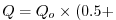 random number between 0 and 1 random number between 0 and 1 .
.
In the example  W m
W m so that values of
lie in the range 400 to
1200 W m
with a mean of
so that values of
lie in the range 400 to
1200 W m
with a mean of  . Although the flux models a loss, because it is
directed upwards, according to the model's sign convention,
is positive.
. Although the flux models a loss, because it is
directed upwards, according to the model's sign convention,
is positive.
Next: 3.15.6 Running the example
Up: 3.15 Surface Driven Convection
Previous: 3.15.4 Numerical stability criteria
Contents
mitgcm-support@mitgcm.org
| Copyright © 2006
Massachusetts Institute of Technology |
Last update 2018-01-23 |
 |
|


