|
|
|
|


Next: 3.19.2 Code configuration
Up: 3.19 Sensitivity of Air-Sea
Previous: 3.19 Sensitivity of Air-Sea
Contents
Subsections
We describe an adjoint sensitivity analysis of out-gassing from
the ocean into the atmosphere of a carbon-like tracer injected
into the ocean interior (see Hill et al. [2002]).
For this work MITgcm was augmented with a thermodynamically
inactive tracer,  . Tracer residing in the ocean
model surface layer is out-gassed according to a relaxation time scale,
. Tracer residing in the ocean
model surface layer is out-gassed according to a relaxation time scale,
 . Within the ocean interior, the tracer is passively advected
by the ocean model currents. The full equation for the time evolution
. Within the ocean interior, the tracer is passively advected
by the ocean model currents. The full equation for the time evolution
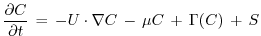 |
(3.93) |
also includes a source term  . This term
represents interior sources of
such as would arise due to
direct injection.
The velocity term,
. This term
represents interior sources of
such as would arise due to
direct injection.
The velocity term,  , is the sum of the
model Eulerian circulation and an eddy-induced velocity, the latter
parameterized according to Gent/McWilliams
(Gent and McWilliams [1990]; Gent et al. [1995]).
The convection function,
, is the sum of the
model Eulerian circulation and an eddy-induced velocity, the latter
parameterized according to Gent/McWilliams
(Gent and McWilliams [1990]; Gent et al. [1995]).
The convection function,  , mixes
vertically wherever the
fluid is locally statically unstable.
, mixes
vertically wherever the
fluid is locally statically unstable.
The out-gassing time scale,
, in eqn. (3.94)
is set so that
 for the surface
ocean and
for the surface
ocean and  elsewhere. With this value, eqn. (3.94)
is valid as a prognostic equation for small perturbations in oceanic
carbon concentrations. This configuration provides a
powerful tool for examining the impact of large-scale ocean circulation
on
elsewhere. With this value, eqn. (3.94)
is valid as a prognostic equation for small perturbations in oceanic
carbon concentrations. This configuration provides a
powerful tool for examining the impact of large-scale ocean circulation
on  out-gassing due to interior injections.
As source we choose a constant in time injection of
out-gassing due to interior injections.
As source we choose a constant in time injection of
 .
.
The model configuration employed has a constant
 resolution horizontal grid and realistic
geography and bathymetry. Twenty vertical layers are used with
vertical spacing ranging
from 50 m near the surface to 815 m at depth.
Driven to steady-state by climatological wind-stress, heat and
fresh-water forcing the model reproduces well known large-scale
features of the ocean general circulation.
resolution horizontal grid and realistic
geography and bathymetry. Twenty vertical layers are used with
vertical spacing ranging
from 50 m near the surface to 815 m at depth.
Driven to steady-state by climatological wind-stress, heat and
fresh-water forcing the model reproduces well known large-scale
features of the ocean general circulation.
To quantify and understand out-gassing due to injections of
in eqn. (3.94),
we define a cost function  that measures the total amount of
tracer out-gassed at each timestep:
that measures the total amount of
tracer out-gassed at each timestep:
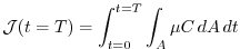 |
(3.94) |
Equation(3.95) integrates the out-gassing term,  ,
from (3.94)
over the entire ocean surface area,
,
from (3.94)
over the entire ocean surface area,  , and accumulates it
up to time
, and accumulates it
up to time  .
Physically,
can be thought of as representing the amount of
that our model predicts would be out-gassed following an
injection at rate
.
The sensitivity of
to the spatial location of
,
.
Physically,
can be thought of as representing the amount of
that our model predicts would be out-gassed following an
injection at rate
.
The sensitivity of
to the spatial location of
,
 ,
can be used to identify regions from which circulation
would cause
to rapidly out-gas following injection
and regions in which
injections would remain effectively
sequestered within the ocean.
,
can be used to identify regions from which circulation
would cause
to rapidly out-gas following injection
and regions in which
injections would remain effectively
sequestered within the ocean.
Next: 3.19.2 Code configuration
Up: 3.19 Sensitivity of Air-Sea
Previous: 3.19 Sensitivity of Air-Sea
Contents
mitgcm-support@mitgcm.org
| Copyright © 2006
Massachusetts Institute of Technology |
Last update 2018-01-23 |
 |
|


