|
|
|
|


Next: 5.2 TLM and ADM
Up: 5.1 Some basic algebra
Previous: 5.1.2 Reverse or adjoint
Contents
5.1.3 Storing vs. recomputation in reverse mode
We note an important aspect of the forward vs. reverse
mode calculation.
Because of the local character of the derivative
(a derivative is defined w.r.t. a point along the trajectory),
the intermediate results of the model trajectory
 may be required to evaluate the intermediate Jacobian
 .
This is the case e.g. for nonlinear expressions
(momentum advection, nonlinear equation of state), state-dependent
conditional statements (parameterization schemes).
In the forward mode, the intermediate results are required
in the same order as computed by the full forward model
.
This is the case e.g. for nonlinear expressions
(momentum advection, nonlinear equation of state), state-dependent
conditional statements (parameterization schemes).
In the forward mode, the intermediate results are required
in the same order as computed by the full forward model  ,
but in the reverse mode they are required in the reverse order.
Thus, in the reverse mode the trajectory of the forward model
integration
has to be stored to be available in the reverse
calculation. Alternatively, the complete model state up to the
point of evaluation has to be recomputed whenever its value is required.
,
but in the reverse mode they are required in the reverse order.
Thus, in the reverse mode the trajectory of the forward model
integration
has to be stored to be available in the reverse
calculation. Alternatively, the complete model state up to the
point of evaluation has to be recomputed whenever its value is required.
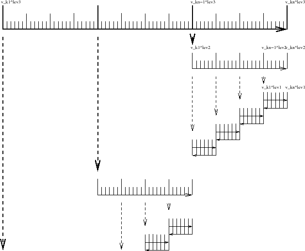
A method to balance the amount of recomputations vs.
storage requirements is called checkpointing
(e.g. Griewank [1992], Restrepo et al. [1998]).
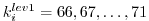
It is depicted in 5.1 for a 3-level checkpointing
[as an example, we give explicit numbers for a 3-day
integration with a 1-hourly timestep in square brackets].

- In a first step, the model trajectory is subdivided into
 subsections [
=3 1-day intervals],
with the label
for this outermost loop.
The model is then integrated along the full trajectory,
and the model state stored to disk only at every
subsections [
=3 1-day intervals],
with the label
for this outermost loop.
The model is then integrated along the full trajectory,
and the model state stored to disk only at every
 -th timestep
[i.e. 3 times, at
-th timestep
[i.e. 3 times, at
 corresponding to
 ].
In addition, the cost function is computed, if needed.
].
In addition, the cost function is computed, if needed.

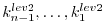
- In a second step each subsection itself is divided into
 subsections
[
=4 6-hour intervals per subsection].
The model picks up at the last outermost dumped state
subsections
[
=4 6-hour intervals per subsection].
The model picks up at the last outermost dumped state
 and is integrated forward in time along
the last subsection, with the label
for this
intermediate loop.
The model state is now stored to disk at every
and is integrated forward in time along
the last subsection, with the label
for this
intermediate loop.
The model state is now stored to disk at every
 -th
timestep
[i.e. 4 times, at
-th
timestep
[i.e. 4 times, at
 corresponding to
 ].
].

- Finally, the model picks up at the last intermediate dump state
 and is integrated forward in time along
the last subsection, with the label
for this
intermediate loop.
Within this sub-subsection only, parts of the model state is stored
to memory at every timestep
[i.e. every hour
and is integrated forward in time along
the last subsection, with the label
for this
intermediate loop.
Within this sub-subsection only, parts of the model state is stored
to memory at every timestep
[i.e. every hour  corresponding to
 ].
The final state
].
The final state
 is reached
and the model state of all preceding timesteps along the last
innermost subsection are available, enabling integration backwards
in time along the last subsection.
The adjoint can thus be computed along this last
subsection
is reached
and the model state of all preceding timesteps along the last
innermost subsection are available, enabling integration backwards
in time along the last subsection.
The adjoint can thus be computed along this last
subsection
 .
.
This procedure is repeated consecutively for each previous
subsection
 carrying the adjoint computation to the initial time
of the subsection
carrying the adjoint computation to the initial time
of the subsection
 .
Then, the procedure is repeated for the previous subsection
.
Then, the procedure is repeated for the previous subsection
 carrying the adjoint computation to the initial time
 .
.
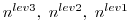
For the full model trajectory of
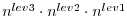 timesteps
the required storing of the model state was significantly reduced to
timesteps
the required storing of the model state was significantly reduced to
 to disk and roughly
  to memory
[i.e. for the 3-day integration with a total oof 72 timesteps
the model state was stored 7 times to disk and roughly 6 times
to memory].
This saving in memory comes at a cost of a required
3 full forward integrations of the model (one for each
checkpointing level).
The optimal balance of storage vs. recomputation certainly depends
on the computing resources available and may be adjusted by
adjusting the partitioning among the
to memory
[i.e. for the 3-day integration with a total oof 72 timesteps
the model state was stored 7 times to disk and roughly 6 times
to memory].
This saving in memory comes at a cost of a required
3 full forward integrations of the model (one for each
checkpointing level).
The optimal balance of storage vs. recomputation certainly depends
on the computing resources available and may be adjusted by
adjusting the partitioning among the
 .
.
Figure 5.1:
Schematic view of intermediate dump and restart for
3-level checkpointing.
|
|
Next: 5.2 TLM and ADM
Up: 5.1 Some basic algebra
Previous: 5.1.2 Reverse or adjoint
Contents
mitgcm-support@mitgcm.org
| Copyright © 2006
Massachusetts Institute of Technology |
Last update 2018-01-23 |
 |
|