|
|
|
|


Next: 5.1.3 Storing vs. recomputation
Up: 5.1 Some basic algebra
Previous: 5.1.1 Forward or direct
Contents
Subsections
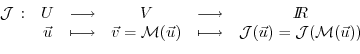
Let us consider the special case of a
scalar objective function
 of the model output (e.g.
the total meridional heat transport,
the total uptake of
of the model output (e.g.
the total meridional heat transport,
the total uptake of  in the Southern
Ocean over a time interval,
or a measure of some model-to-data misfit)
in the Southern
Ocean over a time interval,
or a measure of some model-to-data misfit)
 |
|
|
(5.4) |
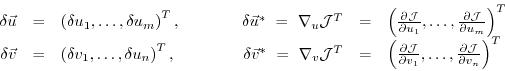
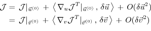
The perturbation of  around a fixed point
 ,
,
can be expressed in both bases of  and
and  w.r.t. their corresponding inner product

(note, that the gradient  is a co-vector, therefore
its transpose is required in the above inner product).
Then, using the representation of
is a co-vector, therefore
its transpose is required in the above inner product).
Then, using the representation of
 ,
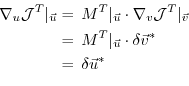
the definition
of an adjoint operator
,
the definition
of an adjoint operator  of a given operator
  ,
,
which for finite-dimensional vector spaces is just the
transpose of
,
and from eq. (5.2), (5.5),
we note that
(omitting  's):
's):
 |
(5.6) |
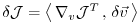
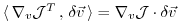
With the identity (5.5), we then find that
the gradient
 can be readily inferred by
invoking the adjoint
can be readily inferred by
invoking the adjoint  of the tangent linear model
Eq. (5.7) is the adjoint model (ADM),
in which  is the adjoint (here, the transpose) of the
tangent linear operator
,
is the adjoint (here, the transpose) of the
tangent linear operator
,
 the adjoint variable of the model state
, and
the adjoint variable of the model state
, and
 the adjoint variable of the control variable
.
the adjoint variable of the control variable
.
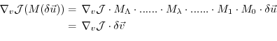
The reverse nature of the adjoint calculation can be readily
seen as follows.
Consider a model integration which consists of  consecutive operations
 ,
where the
,
where the  's could be the elementary steps, i.e. single lines
in the code of the model, or successive time steps of the
model integration,
starting at step 0 and moving up to step
, with intermediate
's could be the elementary steps, i.e. single lines
in the code of the model, or successive time steps of the
model integration,
starting at step 0 and moving up to step
, with intermediate
 and final
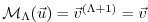 .
Let
be a cost function which explicitly depends on the
final state
only
(this restriction is for clarity reasons only).
.
Let
be a cost function which explicitly depends on the
final state
only
(this restriction is for clarity reasons only).
 may be decomposed according to:
 |
(5.8) |
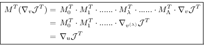
Then, according to the chain rule, the forward calculation reads,
in terms of the Jacobi matrices
(we've omitted the
's which, nevertheless are important
to the aspect of tangent linearity;
note also that by definition
 )
)
whereas in reverse mode we have
clearly expressing the reverse nature of the calculation.
Eq. (5.10) is at the heart of automatic adjoint compilers.
If the intermediate steps  in
eqn. (5.8) - (5.10)
represent the model state (forward or adjoint) at each
intermediate time step as noted above, then correspondingly,
in
eqn. (5.8) - (5.10)
represent the model state (forward or adjoint) at each
intermediate time step as noted above, then correspondingly,
 for the adjoint variables.
It thus becomes evident that the adjoint calculation also
yields the adjoint of each model state component
for the adjoint variables.
It thus becomes evident that the adjoint calculation also
yields the adjoint of each model state component
 at each intermediate step
, namely
at each intermediate step
, namely
in close analogy to eq. (5.7)
We note in passing that that the
 are the Lagrange multipliers of the model equations which determine
.
are the Lagrange multipliers of the model equations which determine
.
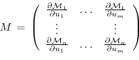
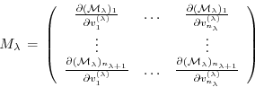
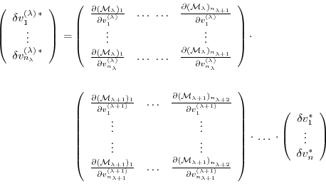
In components, eq. (5.7) reads as follows.
Let
denote the perturbations in
and
, respectively,
and their adjoint variables;
further
is the Jacobi matrix of
(an
 matrix)
such that
matrix)
such that
 , or
, or
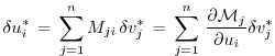
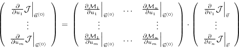
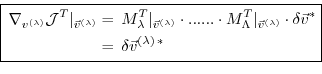
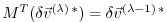
Then eq. (5.7) takes the form
or
Furthermore, the adjoint
 of any intermediate state
 may be obtained, using the intermediate Jacobian
(an
may be obtained, using the intermediate Jacobian
(an
 matrix)
and the shorthand notation for the adjoint variables
 ,
,
 ,
for intermediate components, yielding
,
for intermediate components, yielding
Eq. (5.9) and (5.10) are perhaps clearest in
showing the advantage of the reverse over the forward mode
if the gradient
, i.e. the sensitivity of the
cost function
with respect to all input
variables  (or the sensitivity of the cost function with respect to
all intermediate states
) are sought.
In order to be able to solve for each component of the gradient
(or the sensitivity of the cost function with respect to
all intermediate states
) are sought.
In order to be able to solve for each component of the gradient
 in (5.9)
a forward calculation has to be performed for each component separately,
i.e.
in (5.9)
a forward calculation has to be performed for each component separately,
i.e.
 for the
  -th forward calculation.
Then, (5.9) represents the
projection of
-th forward calculation.
Then, (5.9) represents the
projection of
 onto the
-th component.
The full gradient is retrieved from the
onto the
-th component.
The full gradient is retrieved from the  forward calculations.
In contrast, eq. (5.10) yields the full
gradient
(and all intermediate gradients
forward calculations.
In contrast, eq. (5.10) yields the full
gradient
(and all intermediate gradients
 ) within a single reverse calculation.
Note, that if
is a vector-valued function
of dimension  ,
eq. (5.10) has to be modified according to
,
eq. (5.10) has to be modified according to
where now
 is a vector of
dimension
is a vector of
dimension  .
In this case
reverse simulations have to be performed
for each
.
In this case
reverse simulations have to be performed
for each
 .
Then, the reverse mode is more efficient as long as
.
Then, the reverse mode is more efficient as long as
 , otherwise the forward mode is preferable.
Strictly, the reverse mode is called adjoint mode only for
, otherwise the forward mode is preferable.
Strictly, the reverse mode is called adjoint mode only for
 .
.
A detailed analysis of the underlying numerical operations
shows that the computation of
in this way
requires about 2 to 5 times the computation of the cost function.
Alternatively, the gradient vector could be approximated
by finite differences, requiring
computations
of the perturbed cost function.
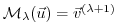
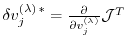
To conclude we give two examples of commonly used types
of cost functions:
The cost function consists of the  -th component of the model state
at time
-th component of the model state
at time  .
Then
.
Then
 is just the
-th
unit vector. The
is just the
-th
unit vector. The
 is the projection of the adjoint
operator onto the
-th component
is the projection of the adjoint
operator onto the
-th component
 ,
,
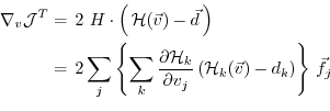
The cost function represents the quadratic model vs. data misfit.
Here,  is the data vector and
  represents the
operator which maps the model state space onto the data space.
Then,
represents the
operator which maps the model state space onto the data space.
Then,
 takes the form
where
 is the
Jacobi matrix of the data projection operator.
Thus, the gradient
is given by the
adjoint operator,
driven by the model vs. data misfit:
is the
Jacobi matrix of the data projection operator.
Thus, the gradient
is given by the
adjoint operator,
driven by the model vs. data misfit:
Next: 5.1.3 Storing vs. recomputation
Up: 5.1 Some basic algebra
Previous: 5.1.1 Forward or direct
Contents
mitgcm-support@mitgcm.org
| Copyright © 2006
Massachusetts Institute of Technology |
Last update 2018-01-23 |
 |
|