|
|
|
|


Next: 5.3 The gradient check
Up: 5.2 TLM and ADM
Previous: 5.2.4 The cost function
Contents
Subsections
5.2.5 The control variables (independent variables)
The control variables are a subset of the model input
(initial conditions, boundary conditions, model parameters).
Here we identify them with the variable  .
All intermediate variables whose derivative w.r.t. control
variables do not vanish are called active variables.
All subroutines whose derivative w.r.t. the control variables
don't vanish are called active routines.
Read and write operations from and to file can be viewed
as variable assignments. Therefore, files to which
active variables are written and from which active variables
are read are called active files.
All aspects relevant to the treatment of the control variables
(parameter setting, initialization, perturbation)
are controlled by the package pkg/ctrl.
.
All intermediate variables whose derivative w.r.t. control
variables do not vanish are called active variables.
All subroutines whose derivative w.r.t. the control variables
don't vanish are called active routines.
Read and write operations from and to file can be viewed
as variable assignments. Therefore, files to which
active variables are written and from which active variables
are read are called active files.
All aspects relevant to the treatment of the control variables
(parameter setting, initialization, perturbation)
are controlled by the package pkg/ctrl.
Figure 5.5:
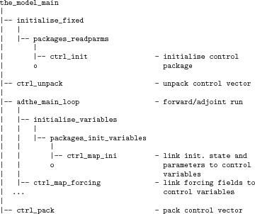 |
To enable the directory to be included to the compile list,
ctrl has to be added to the enable list in
.genmakerc or in genmake itself (analogous to cost
package, cf. previous section).
Each control variable is enabled via its own CPP option
in ECCO_CPPOPTIONS.h.
The dependency flow for differentiation w.r.t. the controls
starts with adding a perturbation onto the input variable,
thus defining the independent or control variables for TAF.
Three types of controls may be considered:
-

Consider as an example the initial tracer distribution
tr1 as control variable.
After tr1 has been initialised in
ini_tr1 (dynamical variables such as
temperature and salinity are initialised in ini_fields),
a perturbation anomaly is added to the field in S/R
ctrl_map_ini
xx_tr1 is a 3-dim. global array
holding the perturbation. In the case of a simple
sensitivity study this array is identical to zero.
However, it's specification is essential in the context
of automatic differentiation since TAF
treats the corresponding line in the code symbolically
when determining the differentiation chain and its origin.
Thus, the variable names are part of the argument list
when calling TAF:
taf -input 'xx_tr1 ...' ...
Now, as mentioned above, MITgcm avoids maintaining
an array for each control variable by reading the
perturbation to a temporary array from file.
To ensure the symbolic link to be recognized by TAF, a scalar
dummy variable xx_tr1_dummy is introduced
and an 'active read' routine of the adjoint support
package pkg/autodiff is invoked.
The read-procedure is tagged with the variable
xx_tr1_dummy enabling TAF to recognize the
initialization of the perturbation.
The modified call of TAF thus reads
taf -input 'xx_tr1_dummy ...' ...
and the modified operation to (5.14)
in the code takes on the form
       call active_read_xyz(
     &      ..., tmpfld3d, ..., xx_tr1_dummy, ... )

       tr1(...) = tr1(...) + tmpfld3d(...)
Note, that reading an active variable corresponds
to a variable assignment. Its derivative corresponds
to a write statement of the adjoint variable, followed by
a reset.
The 'active file' routines have been designed
to support active read and corresponding adjoint active write
operations (and vice versa).
-

The handling of boundary values as control variables
proceeds exactly analogous to the initial values
with the symbolic perturbation taking place in S/R
ctrl_map_forcing.
Note however an important difference:
Since the boundary values are time dependent with a new
forcing field applied at each time steps,
the general problem may be thought of as
a new control variable at each time step
(or, if the perturbation is averaged over a certain period,
at each  timesteps), i.e.
In the current example an equilibrium state is considered,
and only an initial perturbation to
surface forcing is applied with respect to the
equilibrium state.
A time dependent treatment of the surface forcing is
implemented in the ECCO environment, involving the
calendar (cal ) and external forcing (exf ) packages.
-

This routine is not yet implemented, but would proceed
proceed along the same lines as the initial value sensitivity.
The mixing parameters diffkr and kapgm
are currently added as controls in ctrl_map_ini.F.
Several ways exist to generate output of adjoint fields.
-

- xx_...: the control variable fields
Before the forward integration, the control
variables are read from file xx_ ... and added to
the model field.
- adxx_...: the adjoint variable fields, i.e. the gradient
 for each control variable
After the adjoint integration the corresponding adjoint
variables are written to adxx_ ....
-

- vector_ctrl: the control vector
At the very beginning of the model initialization,
the updated compressed control vector is read (or initialised)
and distributed to 2-dim. and 3-dim. control variable fields.
- vector_grad: the gradient vector
At the very end of the adjoint integration,
the 2-dim. and 3-dim. adjoint variables are read,
compressed to a single vector and written to file.
-

In addition to writing the gradient at the end of the
forward/adjoint integration, many more adjoint variables
of the model state
at intermediate times can be written using S/R
addummy_in_stepping.
This routine is part of the adjoint support package
pkg/autodiff (cf.f. below).
The procedure is enabled using via the CPP-option
ALLOW_AUTODIFF_MONITOR (file ECCO_CPPOPTIONS.h).
To be part of the adjoint code, the corresponding S/R
dummy_in_stepping has to be called in the forward
model (S/R the_main_loop) at the appropriate place.
The adjoint common blocks are extracted from the adjoint code
via the header file adcommon.h.
dummy_in_stepping is essentially empty,
the corresponding adjoint routine is hand-written rather
than generated automatically.
Appropriate flow directives (dummy_in_stepping.flow)
ensure that TAMC does not automatically
generate addummy_in_stepping by trying to differentiate
dummy_in_stepping, but instead refers to
the hand-written routine.
dummy_in_stepping is called in the forward code
at the beginning of each
timestep, before the call to dynamics, thus ensuring
that addummy_in_stepping is called at the end of
each timestep in the adjoint calculation, after the call to
addynamics.
addummy_in_stepping includes the header files
adcommon.h.
This header file is also hand-written. It contains
the common blocks
/addynvars_r/, /addynvars_cd/,
/addynvars_diffkr/, /addynvars_kapgm/,
/adtr1_r/, /adffields/,
which have been extracted from the adjoint code to enable
access to the adjoint variables.
WARNING: If the structure of the common blocks
/dynvars_r/, /dynvars_cd/, etc., changes
similar changes will occur in the adjoint common blocks.
Therefore, consistency between the TAMC-generated common blocks
and those in adcommon.h have to be checked.
In optimization mode the cost function
 is sought
to be minimized with respect to a set of control variables
is sought
to be minimized with respect to a set of control variables
 , in an iterative manner.
The gradient
, in an iterative manner.
The gradient
![$ \nabla _{u}{\cal J} \vert _{u_{[k]}} $](img1918.png) together
with the value of the cost function itself
together
with the value of the cost function itself
![$ {\cal J}(u_{[k]}) $](img1919.png) at iteration step
at iteration step  serve
as input to a minimization routine (e.g. quasi-Newton method,
conjugate gradient, ... Gilbert and Lemaréchal [1989])
to compute an update in the
control variable for iteration step
serve
as input to a minimization routine (e.g. quasi-Newton method,
conjugate gradient, ... Gilbert and Lemaréchal [1989])
to compute an update in the
control variable for iteration step 
![$\displaystyle u_{[k+1]} \, = \, u_{[0]} \, + \, \Delta u_{[k+1]}$](img1921.png) satisfying ![$\displaystyle \quad
{\cal J} \left( u_{[k+1]} \right) \, < \, {\cal J} \left( u_{[k]} \right)
$](img1922.png)
![$ u_{[k+1]} $](img1923.png) then serves as input for a forward/adjoint run
to determine
then serves as input for a forward/adjoint run
to determine  and
at iteration step
.
Tab. ref:ask-the-author sketches the flow between forward/adjoint model
and the minimization routine.
and
at iteration step
.
Tab. ref:ask-the-author sketches the flow between forward/adjoint model
and the minimization routine.
The routines ctrl_unpack and ctrl_pack provide
the link between the model and the minimization routine.
As described in Section ref:ask-the-author
the unpack and pack routines read and write
control and gradient vectors which are compressed
to contain only wet points, in addition to the full
2-dim. and 3-dim. fields.
The corresponding I/O flow looks as follows:
vector_ctrl_ k
k
|
|
|
|
|
|
&darr#downarrow; |
|
|
|
|
|
ctrl_unpack |
|
|
|
|
|
&darr#downarrow; |
|
|
|
|
|
xx_theta0...
k
|
|
|
|
|
|
xx_salt0...
k
|

|
forward integration |
|
|
|
&vellip#vdots; |
|
|
|
|
|
|
|

|
|
|
|
|
|
|
|
adxx_theta0...
k
|
|
|
|
adjoint integration |

|
adxx_salt0...
k
|
|
|
|
|
|
&vellip#vdots; |
|
|
|
|
|
&darr#downarrow; |
|
|
|
|
|
ctrl_pack |
|
|
|
|
|
&darr#downarrow; |
|
|
|
|
|
vector_grad_
k
|
ctrl_unpack reads the updated control vector
vector_ctrl_
k
.
It distributes the different control variables to
2-dim. and 3-dim. files xx_...
k
.
At the start of the forward integration the control variables
are read from xx_...
k
and added to the
field.
Correspondingly, at the end of the adjoint integration
the adjoint fields are written
to adxx_...
k
, again via the active file routines.
Finally, ctrl_pack collects all adjoint files
and writes them to the compressed vector file
vector_grad_
k
.
Next: 5.3 The gradient check
Up: 5.2 TLM and ADM
Previous: 5.2.4 The cost function
Contents
mitgcm-support@mitgcm.org
| Copyright © 2006
Massachusetts Institute of Technology |
Last update 2018-01-23 |
 |
|


![\begin{equation*}\begin{aligned}u & = \, u_{[0]} \, + \, \Delta u \\ {\bf tr1}(....
... \, {\bf tr1_{ini}}(...) \, + \, {\bf xx\_tr1}(...) \end{aligned}\end{equation*}](img1909.png)
![\begin{displaymath}\begin{array}{ccccc}
u_{[0]} \,\, , \,\, \Delta u_{[k]} & ~ &...
...downarrow \\
~ & ~ & ~ & ~ & \Delta u_{[k+1]} \\
\end{array}\end{displaymath}](img1924.png)


