 |
 |
|||||||||||
 |
|
|||||||||||
 |
 |
|||||||||||


|
Next: 6.4.8 CAL: The calendar Up: 6.4 Ocean Packages Previous: 6.4.6 BULK_FORCE: Bulk Formula Contents Subsections
|
||||||||||||||||||||||||||||||||||||||||||||||||||||||||||||||||||||||||||||||||||||||||||||||||||||||||||||||||||||||||||||||||||||||||||||||||||||||||||||||||||||||||||||||||||||||||||||||||||||||
|
6.4.7.3.3 Field attributes
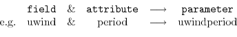
All EXF fields are listed in Section 6.4.7.5. Each field has a number of attributes which can be customized. They are summarized in Table 6.11. To obtain an attribute for a specific field, e.g. uwind prepend the field name to the listed attribute, e.g. for attribute period this yields uwindperiod:
 |
| |||||||||||||||||||||||||||||||||||||||||||||||||||
6.4.7.3.4 Example configuration
The following block is taken from the data.exf file of the verification experiment global_with_exf/. It defines attributes for the heat flux variable hflux:
 hfluxfile       = 'ncep_qnet.bin',
 hfluxstartdate1 = 19920101,
 hfluxstartdate2 = 000000,
 hfluxperiod     = 2592000.0,
 hflux_lon0      = 2
 hflux_lon_inc   = 4
 hflux_lat0      = -78
 hflux_lat_inc   = 39*4
 hflux_nlon      = 90
 hflux_nlat      = 40
EXF will read a file of name 'ncep_qnet.bin'. Its first record represents January 1st, 1992 at 00:00 UTC. Next record is 2592000 seconds (or 30 days) later. Note that the first record read and used by the EXF package corresponds to the value 'startDate1' set in data.cal. Therefore if you want to start the EXF forcing from later in the 'ncep_qnet.bin' file, it suffices to specify startDate1 in data.cal as a date later than 19920101 (for example, startDate1 = 19940101, for starting January 1st, 1994). For this to work, 'ncep_qnet.bin' must have at least 2 years of data because in this configuration EXF will read 2 years into the file to find the 1994 starting value. Interpolation on-the-fly is used (in the present case trivially on the same grid, but included nevertheless for illustration), and input field grid starting coordinates and increments are supplied as well.
6.4.7.4 EXF bulk formulae
T.B.D. (cross-ref. to parameter list table)
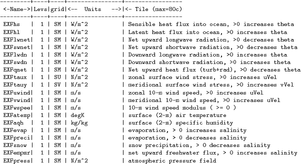
6.4.7.5 EXF input fields and units
The following list is taken from the header file EXF_FIELDS.h. It comprises all EXF input fields.
Output fields which EXF provides to the MITgcm are fields fu, fv, Qnet, Qsw, EmPmR, and pload. They are defined in FFIELDS.h.
c----------------------------------------------------------------------
c               |
c     field     :: Description
c               |
c----------------------------------------------------------------------
c     ustress   :: Zonal surface wind stress in N/m^2
c               |  > 0 for increase in uVel, which is west to
c               |      east for cartesian and spherical polar grids
c               |  Typical range: -0.5 < ustress < 0.5
c               |  Southwest C-grid U point
c               |  Input field
c----------------------------------------------------------------------
c     vstress   :: Meridional surface wind stress in N/m^2
c               |  > 0 for increase in vVel, which is south to
c               |      north for cartesian and spherical polar grids
c               |  Typical range: -0.5 < vstress < 0.5
c               |  Southwest C-grid V point
c               |  Input field
c----------------------------------------------------------------------
c     hs        :: sensible heat flux into ocean in W/m^2
c               |  > 0 for increase in theta (ocean warming)
c----------------------------------------------------------------------
c     hl        :: latent   heat flux into ocean in W/m^2
c               |  > 0 for increase in theta (ocean warming)
c----------------------------------------------------------------------
c     hflux     :: Net upward surface heat flux in W/m^2
c               |  (including shortwave)
c               |  hflux = latent + sensible + lwflux + swflux
c               |  > 0 for decrease in theta (ocean cooling)
c               |  Typical range: -250 < hflux < 600
c               |  Southwest C-grid tracer point
c               |  Input field
c----------------------------------------------------------------------
c     sflux     :: Net upward freshwater flux in m/s
c               |  sflux = evap - precip - runoff
c               |  > 0 for increase in salt (ocean salinity)
c               |  Typical range: -1e-7 < sflux < 1e-7
c               |  Southwest C-grid tracer point
c               |  Input field
c----------------------------------------------------------------------
c     swflux    :: Net upward shortwave radiation in W/m^2
c               |  swflux = - ( swdown - ice and snow absorption - reflected )
c               |  > 0 for decrease in theta (ocean cooling)
c               |  Typical range: -350 < swflux < 0
c               |  Southwest C-grid tracer point
c               |  Input field
c----------------------------------------------------------------------
c     uwind     :: Surface (10-m) zonal wind velocity in m/s
c               |  > 0 for increase in uVel, which is west to
c               |      east for cartesian and spherical polar grids
c               |  Typical range: -10 < uwind < 10
c               |  Southwest C-grid U point
c               |  Input or input/output field
c----------------------------------------------------------------------
c     vwind     :: Surface (10-m) meridional wind velocity in m/s
c               |  > 0 for increase in vVel, which is south to
c               |      north for cartesian and spherical polar grids
c               |  Typical range: -10 < vwind < 10
c               |  Southwest C-grid V point
c               |  Input or input/output field
c----------------------------------------------------------------------
c     wspeed    :: Surface (10-m) wind speed in m/s
c               |  >= 0 sqrt(u^2+v^2)
c               |  Typical range: 0 < wspeed < 10
c               |  Input or input/output field
c----------------------------------------------------------------------
c     atemp     :: Surface (2-m) air temperature in deg K
c               |  Typical range: 200 < atemp < 300
c               |  Southwest C-grid tracer point
c               |  Input or input/output field
c----------------------------------------------------------------------
c     aqh       :: Surface (2m) specific humidity in kg/kg
c               |  Typical range: 0 < aqh < 0.02
c               |  Southwest C-grid tracer point
c               |  Input or input/output field
c----------------------------------------------------------------------
c     lwflux    :: Net upward longwave radiation in W/m^2
c               |  lwflux = - ( lwdown - ice and snow absorption - emitted )
c               |  > 0 for decrease in theta (ocean cooling)
c               |  Typical range: -20 < lwflux < 170
c               |  Southwest C-grid tracer point
c               |  Input field
c----------------------------------------------------------------------
c     evap      :: Evaporation in m/s
c               |  > 0 for increase in salt (ocean salinity)
c               |  Typical range: 0 < evap < 2.5e-7
c               |  Southwest C-grid tracer point
c               |  Input, input/output, or output field
c----------------------------------------------------------------------
c     precip    :: Precipitation in m/s
c               |  > 0 for decrease in salt (ocean salinity)
c               |  Typical range: 0 < precip < 5e-7
c               |  Southwest C-grid tracer point
c               |  Input or input/output field
c----------------------------------------------------------------------
c    snowprecip :: snow in m/s
c               |  > 0 for decrease in salt (ocean salinity)
c               |  Typical range: 0 < precip < 5e-7
c               |  Input or input/output field
c----------------------------------------------------------------------
c     runoff    :: River and glacier runoff in m/s
c               |  > 0 for decrease in salt (ocean salinity)
c               |  Typical range: 0 < runoff < ????
c               |  Southwest C-grid tracer point
c               |  Input or input/output field
c               |  !!! WATCH OUT: Default exf_inscal_runoff !!!
c               |  !!! in exf_readparms.F is not 1.0        !!!
c----------------------------------------------------------------------
c     swdown    :: Downward shortwave radiation in W/m^2
c               |  > 0 for increase in theta (ocean warming)
c               |  Typical range: 0 < swdown < 450
c               |  Southwest C-grid tracer point
c               |  Input/output field
c----------------------------------------------------------------------
c     lwdown    :: Downward longwave radiation in W/m^2
c               |  > 0 for increase in theta (ocean warming)
c               |  Typical range: 50 < lwdown < 450
c               |  Southwest C-grid tracer point
c               |  Input/output field
c----------------------------------------------------------------------
c     apressure :: Atmospheric pressure field in N/m^2
c               |  > 0 for ????
c               |  Typical range: ???? < apressure < ????
c               |  Southwest C-grid tracer point
c               |  Input field
c----------------------------------------------------------------------
6.4.7.6 Key subroutines
Top-level routine: exf_getforcing.F
C     !CALLING SEQUENCE:
c ...
c  exf_getforcing (TOP LEVEL ROUTINE)
c  |
c  |-- exf_getclim (get climatological fields used e.g. for relax.)
c  |   |--- exf_set_climsst  (relax. to 2-D SST field)
c  |   |--- exf_set_climsss  (relax. to 2-D SSS field)
c  |   o
c  |
c  |-- exf_getffields <- this one does almost everything
c  |   |   1. reads in fields, either flux or atmos. state,
c  |   |      depending on CPP options (for each variable two fields
c  |   |      consecutive in time are read in and interpolated onto
c  |   |      current time step).
c  |   |   2. If forcing is atmos. state and control is atmos. state,
c  |   |      then the control variable anomalies are read here via ctrl_get_gen
c  |   |      (atemp, aqh, precip, swflux, swdown, uwind, vwind).
c  |   |      If forcing and control are fluxes, then
c  |   |      controls are added later.
c  |   o
c  |
c  |-- exf_radiation
c  |   |    Compute net or downwelling radiative fluxes via
c  |   |    Stefan-Boltzmann law in case only one is known.
c  |   o
c  |-- exf_wind
c  |   |   Computes wind speed and stresses, if required.
c  |   o
c  |
c  |-- exf_bulkformulae
c  |   |   Compute air-sea buoyancy fluxes from
c  |   |   atmospheric state following Large and Pond, JPO, 1981/82
c  |   o
c  |
c  |-- < hflux is sum of sensible, latent, longwave rad. >
c  |-- < sflux is sum of evap. minus precip. minus runoff  >
c  |
c  |-- exf_getsurfacefluxes
c  |   If forcing and control is flux, then the
c  |   control vector anomalies are read here via ctrl_get_gen
c  |   (hflux, sflux, ustress, vstress)
c  |
c  |-- < update tile edges here >
c  |
c  |-- exf_check_range
c  |   |   Check whether read fields are within assumed range
c  |   |   (may capture mismatches in units)
c  |   o
c  |
c  |-- < add shortwave to hflux for diagnostics >
c  |
c  |-- exf_diagnostics_fill
c  |   |   Do EXF-related diagnostics output here.
c  |   o
c  |
c  |-- exf_mapfields
c  |   |   Forcing fields from exf package are mapped onto
c  |   |   mitgcm forcing arrays.
c  |   |   Mapping enables a runtime rescaling of fields
c  |   o
C  o
Radiation calculation: exf_radiation.F
Wind speed and stress calculation: exf_wind.F
Bulk formula: exf_bulkformulae.F
Generic I/O: exf_set_gen.F
Interpolation: exf_interp.F
Header routines
6.4.7.7 EXF diagnostics
Diagnostics output is available via the diagnostics package (see Section 7.1). Available output fields are summarized in Table 6.12.
6.4.7.8 Experiments and tutorials that use exf
- Global Ocean experiment, in global_with_exf verification directory
- Labrador Sea experiment, in lab_sea verification directory
6.4.7.9 References
Next: 6.4.8 CAL: The calendar Up: 6.4 Ocean Packages Previous: 6.4.6 BULK_FORCE: Bulk Formula Contents mitgcm-support@mitgcm.org
| Copyright © 2006 Massachusetts Institute of Technology | Last update 2018-01-23 |


