|
|
|
|


Next: 1.5 Appendix OCEAN
Up: 1.4 Appendix ATMOSPHERE
Previous: 1.4 Appendix ATMOSPHERE
Contents
Subsections
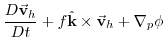
The hydrostatic primitive equations (HPEs) in p-coordinates are:
 |
 |
 |
(1.45) |
 |
|
0 |
(1.46) |
 |
|
0 |
(1.47) |
 |
|
 |
(1.48) |
 |
|
 |
(1.49) |
where
 is the `horizontal' (on pressure
surfaces) component of velocity,
is the `horizontal' (on pressure
surfaces) component of velocity,
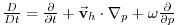 is the total derivative,
 is the Coriolis parameter,
 is the geopotential,
 is the specific volume,
 is the vertical velocity in the
  coordinate.
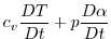
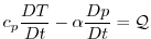
Equation(1.49) is the first law of thermodynamics where internal
energy
coordinate.
Equation(1.49) is the first law of thermodynamics where internal
energy  ,
,  is temperature,
  is the rate of heating per unit mass
and
is the rate of heating per unit mass
and
 is the work done by the fluid in compressing.
It is convenient to cast the heat equation in terms of potential temperature
 so that it looks more like a generic conservation law.
Differentiating (1.48) we get:
so that it looks more like a generic conservation law.
Differentiating (1.48) we get:
which, when added to the heat equation (1.49) and using
 , gives:
 |
(1.50) |
Potential temperature is defined:
 |
(1.51) |
where  is a reference pressure and
 . For convenience
we will make use of the Exner function
. For convenience
we will make use of the Exner function  which defined by:
 |
(1.52) |
The following relations will be useful and are easily expressed in terms of
the Exner function:
where
 is the buoyancy.
The heat equation is obtained by noting that
and on substituting into (1.50) gives:
 |
(1.53) |
which is in conservative form.
For convenience in the model we prefer to step forward (1.53) rather than (1.49).
The upper and lower boundary conditions are :
at the top: |
|
,  |
(1.54) |
at the surface: |
|
,  |
(1.55) |
In  -coordinates, the upper boundary acts like a solid boundary (
 ); in
); in  -coordinates and the lower boundary is analogous to a free
surface (
-coordinates and the lower boundary is analogous to a free
surface ( is imposed and
 ).
).
1.4.1.2 Splitting the geo-potential
For the purposes of initialization and reducing round-off errors, the model
deals with perturbations from reference (or ``standard'') profiles. For
example, the hydrostatic geopotential associated with the resting atmosphere
is not dynamically relevant and can therefore be subtracted from the
equations. The equations written in terms of perturbations are obtained by
substituting the following definitions into the previous model equations:
The reference state (indicated by subscript ``0'') corresponds to
horizontally homogeneous atmosphere at rest (
 ) with surface pressure
 that satisfies
 , defined:
The final form of the HPE's in p coordinates is then:
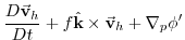 |
|
|
(1.59) |
 |
|
0 |
(1.60) |
|
|
0 |
(1.61) |
 |
|
 |
(1.62) |
 |
|
 |
(1.63) |
Next: 1.5 Appendix OCEAN
Up: 1.4 Appendix ATMOSPHERE
Previous: 1.4 Appendix ATMOSPHERE
Contents
mitgcm-support@mitgcm.org
| Copyright © 2006
Massachusetts Institute of Technology |
Last update 2018-01-23 |
 |
|


