 |
 |
|||||||||||
 |
|
|||||||||||
 |
 |
|||||||||||


|
Next: 6.6 Sea Ice Packages Up: 6.5 Atmosphere Packages Previous: 6.5.2 Land package Contents Subsections
|
||||||||||||||||||||||||||||||||||||||||||||||||||||||||||||||||||||||||||||||||||||||||||||||||||||||||||||||||||||||||||||||||||||||||||||||||||||||||||||||||||||||||||||||||||||||||||||||||||||||||||||||||||||||||||||||||||||||||||||||||||||||||||||||||||||||||||||||||||||||||||||||||||||||||||||||||||||||||||||||||||||||||||||||||||||||||||||||||||||||||||||||||||||||||||||||||||||||||||||||||||||||||||||||||||||||||||||||||||||||||||||||||||||||||||||||||||||||||||||||||||||||||||||||||||||||||||||||||||||||||||||||||||||||||||||||||||||||||||||||||||||||||||||||||||||||||||||||||||||||||||||||||||||||||||||||||||||||||||||||||||||||||||||||||||||||||||||||||||||||||||||||||||||||||||||||||||||||||||||||||||||||||||||||||||||||||||||||||||||||||||||||||||||||||||||||||||||||||||||||||||||||||||||||||||||||||||||||||||||||||||||||
![$\displaystyle F_{LS} = \min\left[ { \left( \frac{RH-RH_c}{1-RH_c} \right) }^2, 1.0 \right]
$](img2255.png)
These cloud fractions are suppressed, however, in regions where the convective
sub-cloud layer is conditionally unstable. The functional form of ![]() is shown in
Figure (6.9).
is shown in
Figure (6.9).
![\begin{figure*}
% latex2html id marker 32493
\vspace{0.4in}
\centerline{ \epsf...
...ive Humidity for Clouds.] {Critical Relative Humidity for Clouds.}
\end{figure*}](img2264.png)
The total cloud fraction in a grid box is determined by the larger of the two cloud fractions:
Finally, cloud fractions are time-averaged between calls to the radiation packages.
Radiation:
The parameterization of radiative heating in the fizhi package includes effects from both shortwave and longwave processes. Radiative fluxes are calculated at each model edge-level in both up and down directions. The heating rates/cooling rates are then obtained from the vertical divergence of the net radiative fluxes.
The net flux is
where
The heating rate due to the divergence of the radiative flux is given by
or
where
The time tendency for Longwave
Radiation is updated every 3 hours. The time tendency for Shortwave Radiation is updated once
every three hours assuming a normalized incident solar radiation, and subsequently modified at
every model time step by the true incident radiation.
The solar constant value used in the package is equal to 1365 ![]() and a
and a ![]() mixing ratio of 330 ppm.
For the ozone mixing ratio, monthly mean zonally averaged
climatological values specified as a function
of latitude and height (Rosenfield et al. [1987]) are linearly interpolated to the current time.
mixing ratio of 330 ppm.
For the ozone mixing ratio, monthly mean zonally averaged
climatological values specified as a function
of latitude and height (Rosenfield et al. [1987]) are linearly interpolated to the current time.
6.5.3.2.3 Shortwave Radiation
The shortwave radiation package used in the package computes solar radiative heating due to the absoption by water vapor, ozone, carbon dioxide, oxygen, clouds, and aerosols and due to the scattering by clouds, aerosols, and gases. The shortwave radiative processes are described by Chou [1990,1992]. This shortwave package uses the Delta-Eddington approximation to compute the bulk scattering properties of a single layer following King and Harshvardhan (JAS, 1986). The transmittance and reflectance of diffuse radiation follow the procedures of Sagan and Pollock (JGR, 1967) and Lacis and Hansen [1974].
Highly accurate heating rate calculations are obtained through the use of an optimal grouping strategy of spectral bands. By grouping the UV and visible regions as indicated in Table 6.13, the Rayleigh scattering and the ozone absorption of solar radiation can be accurately computed in the ultraviolet region and the photosynthetically active radiation (PAR) region. The computation of solar flux in the infrared region is performed with a broadband parameterization using the spectrum regions shown in Table 6.14. The solar radiation algorithm used in the fizhi package can be applied not only for climate studies but also for studies on the photolysis in the upper atmosphere and the photosynthesis in the biosphere.
|
Infrared Spectral Regions
|
Within the shortwave radiation package, both ice and liquid cloud particles are allowed to co-exist in any of the model layers. Two sets of cloud parameters are used, one for ice paticles and the other for liquid particles. Cloud parameters are defined as the cloud optical thickness and the effective cloud particle size. In the fizhi package, the effective radius for water droplets is given as 10 microns, while 65 microns is used for ice particles. The absorption due to aerosols is currently set to zero.
To simplify calculations in a cloudy atmosphere, clouds are
grouped into low (![]() mb), middle (700 mb
mb), middle (700 mb
![]() mb), and high (
mb), and high (![]() mb) cloud regions.
Within each of the three regions, clouds are assumed maximally
overlapped, and the cloud cover of the group is the maximum
cloud cover of all the layers in the group. The optical thickness
of a given layer is then scaled for both the direct (as a function of the
solar zenith angle) and diffuse beam radiation
so that the grouped layer reflectance is the same as the original reflectance.
The solar flux is computed for each of eight cloud realizations possible within this
low/middle/high classification, and appropriately averaged to produce the net solar flux.
mb) cloud regions.
Within each of the three regions, clouds are assumed maximally
overlapped, and the cloud cover of the group is the maximum
cloud cover of all the layers in the group. The optical thickness
of a given layer is then scaled for both the direct (as a function of the
solar zenith angle) and diffuse beam radiation
so that the grouped layer reflectance is the same as the original reflectance.
The solar flux is computed for each of eight cloud realizations possible within this
low/middle/high classification, and appropriately averaged to produce the net solar flux.
6.5.3.2.4 Longwave Radiation
The longwave radiation package used in the fizhi package is thoroughly described by Chou and M.J.Suarez [1994]. As described in that document, IR fluxes are computed due to absorption by water vapor, carbon dioxide, and ozone. The spectral bands together with their absorbers and parameterization methods, configured for the fizhi package, are shown in Table 6.15.
|
IR Spectral Bands
| ||||||||||||||||||||||||||||||||||||||||||||||||||||||||||||||||||||||||
The longwave radiation package accurately computes cooling rates for the middle and
lower atmosphere from 0.01 mb to the surface. Errors are ![]() 0.4 C day
0.4 C day![]() in cooling
rates and
in cooling
rates and ![]() 1% in fluxes. From Chou and Suarez, it is estimated that the total effect of
neglecting all minor absorption bands and the effects of minor infrared absorbers such as
nitrous oxide (N
1% in fluxes. From Chou and Suarez, it is estimated that the total effect of
neglecting all minor absorption bands and the effects of minor infrared absorbers such as
nitrous oxide (N![]() O), methane (CH
O), methane (CH![]() ), and the chlorofluorocarbons (CFCs), is an underestimate
of
), and the chlorofluorocarbons (CFCs), is an underestimate
of ![]() 5 W/m
5 W/m![]() in the downward flux at the surface and an overestimate of
in the downward flux at the surface and an overestimate of ![]() 3 W/m
3 W/m![]() in the upward flux at the top of the atmosphere.
in the upward flux at the top of the atmosphere.
Similar to the procedure used in the shortwave radiation package, clouds are grouped into
three regions catagorized as low/middle/high.
The net clear line-of-site probability ![]() between any two levels,
between any two levels, ![]() and
and
![]() ,
assuming randomly overlapped cloud groups, is simply the product of the probabilities within each group:
,
assuming randomly overlapped cloud groups, is simply the product of the probabilities within each group:
Since all clouds within a group are assumed maximally overlapped, the clear line-of-site probability within a group is given by:
where ![]() is the maximum cloud fraction encountered between
is the maximum cloud fraction encountered between ![]() and
and ![]() within that group.
For groups and/or levels outside the range of
within that group.
For groups and/or levels outside the range of ![]() and
and ![]() , a clear line-of-site probability equal to 1 is
assigned.
, a clear line-of-site probability equal to 1 is
assigned.
6.5.3.2.5 Cloud-Radiation Interaction
The cloud fractions and diagnosed cloud liquid water produced by moist processes
within the fizhi package are used in the radiation packages to produce cloud-radiative forcing.
The cloud optical thickness associated with large-scale cloudiness is made
proportional to the diagnosed large-scale liquid water, ![]() , detrained due to super-saturation.
Two values are used corresponding to cloud ice particles and water droplets.
The range of optical thickness for these clouds is given as
, detrained due to super-saturation.
Two values are used corresponding to cloud ice particles and water droplets.
The range of optical thickness for these clouds is given as
The partitioning, ![]() , between ice particles and water droplets is achieved through a linear scaling
in temperature:
, between ice particles and water droplets is achieved through a linear scaling
in temperature:
The resulting optical depth associated with large-scale cloudiness is given as
The optical thickness associated with sub-grid scale convective clouds produced by RAS is given as
The total optical depth in a given model layer is computed as a weighted average between the large-scale and sub-grid scale optical depths, normalized by the total cloud fraction in the layer:
where ![]() and
and ![]() are the time-averaged cloud fractions associated with RAS and large-scale
processes described in Section 6.5.3.2.
The optical thickness for the longwave radiative feedback is assumed to be 75
are the time-averaged cloud fractions associated with RAS and large-scale
processes described in Section 6.5.3.2.
The optical thickness for the longwave radiative feedback is assumed to be 75 ![]() of these values.
of these values.
The entire Moist Convective Processes Module is called with a frequency of 10 minutes. The cloud fraction values are time-averaged over the period between Radiation calls (every 3 hours). Therefore, in a time-averaged sense, both convective and large-scale cloudiness can exist in a given grid-box.
6.5.3.2.6 Turbulence
:Turbulence is parameterized in the fizhi package to account for its contribution to the vertical exchange of heat, moisture, and momentum. The turbulence scheme is invoked every 30 minutes, and employs a backward-implicit iterative time scheme with an internal time step of 5 minutes. The tendencies of atmospheric state variables due to turbulent diffusion are calculated using the diffusion equations:
Within the atmosphere, the time evolution of second turbulent moments is explicitly modeled by representing the third moments in terms of the first and second moments. This approach is known as a second-order closure modeling. To simplify and streamline the computation of the second moments, the level 2.5 assumption of Mellor and Yamada (1974) and Yamada [1977] is employed, in which only the turbulent kinetic energy (TKE),
is solved prognostically and the other second moments are solved diagnostically.
The prognostic equation for TKE allows the scheme to simulate
some of the transient and diffusive effects in the turbulence. The TKE budget equation
is solved numerically using an implicit backward computation of the terms linear in ![]() and is written:
and is written:
where ![]() is the turbulent velocity,
is the turbulent velocity,
![]() ,
,
![]() ,
,
![]() and
and
![]() are the fluctuating parts of the velocity components and potential
temperature,
are the fluctuating parts of the velocity components and potential
temperature, ![]() and
and ![]() are the mean velocity components,
are the mean velocity components,
![]() is the
coefficient of thermal expansion, and
is the
coefficient of thermal expansion, and
![]() and
and
![]() are constant
multiples of the master length scale,
are constant
multiples of the master length scale, ![]() , which is designed to be a characteristic measure
of the vertical structure of the turbulent layers.
, which is designed to be a characteristic measure
of the vertical structure of the turbulent layers.
The first term on the left-hand side represents the time rate of change of TKE, and the second term is a representation of the triple correlation, or turbulent transport term. The first three terms on the right-hand side represent the sources of TKE due to shear and bouyancy, and the last term on the right hand side is the dissipation of TKE.
In the level 2.5 approach, the vertical fluxes of the scalars ![]() and
and ![]() and the
wind components
and the
wind components ![]() and
and ![]() are expressed in terms of the diffusion coefficients
are expressed in terms of the diffusion coefficients ![]() and
and
![]() , respectively. In the statisically realizable level 2.5 turbulence scheme of
Helfand and Labraga [1988], these diffusion coefficients are expressed as
, respectively. In the statisically realizable level 2.5 turbulence scheme of
Helfand and Labraga [1988], these diffusion coefficients are expressed as
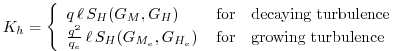
and
where the subscript ![]() refers to the value under conditions of local equillibrium
(obtained from the Level 2.0 Model),
refers to the value under conditions of local equillibrium
(obtained from the Level 2.0 Model), ![]() is the master length scale related to the
vertical structure of the atmosphere,
and
is the master length scale related to the
vertical structure of the atmosphere,
and ![]() and
and ![]() are functions of
are functions of ![]() and
and ![]() , the dimensionless buoyancy and
wind shear parameters, respectively.
Both
, the dimensionless buoyancy and
wind shear parameters, respectively.
Both ![]() and
and ![]() , and their equilibrium values
, and their equilibrium values ![]() and
and ![]() ,
are functions of the Richardson number:
,
are functions of the Richardson number:
Negative values indicate unstable buoyancy and shear, small positive values (![]() )
indicate dominantly unstable shear, and large positive values indicate dominantly stable
stratification.
)
indicate dominantly unstable shear, and large positive values indicate dominantly stable
stratification.
Turbulent eddy diffusion coefficients of momentum, heat and moisture in the surface layer, which corresponds to the lowest GCM level (see -- missing table --), are calculated using stability-dependant functions based on Monin-Obukhov theory:
and
where
![]() is the dimensionless exchange coefficient for momentum from the surface layer
similarity functions:
is the dimensionless exchange coefficient for momentum from the surface layer
similarity functions:
where k is the Von Karman constant and
Here
![]() is the dimensionless exchange coefficient for heat and
moisture from the surface layer similarity functions:
is the dimensionless exchange coefficient for heat and
moisture from the surface layer similarity functions:
where
Here
![]() is the non-dimensional temperature or moisture gradient in the viscous sublayer,
which is the mosstly laminar region between the surface and the tops of the roughness
elements, in which temperature and moisture gradients can be quite large.
Based on Yaglom and Kader [1974]:
is the non-dimensional temperature or moisture gradient in the viscous sublayer,
which is the mosstly laminar region between the surface and the tops of the roughness
elements, in which temperature and moisture gradients can be quite large.
Based on Yaglom and Kader [1974]:
where Pr is the Prandtl number for air,
The surface roughness length over oceans is is a function of the surface-stress velocity,
where the constants are chosen to interpolate between the reciprocal relation of Kondo [1975] for weak winds, and the piecewise linear relation of Large and Pond [1981] for moderate to large winds. Roughness lengths over land are specified from the climatology of Dorman and Sellers [1989].
For an unstable surface layer, the stability functions, chosen to interpolate between the
condition of small values of ![]() and the convective limit, are the KEYPS function
(Panofsky [1973]) for momentum, and its generalization for heat and moisture:
and the convective limit, are the KEYPS function
(Panofsky [1973]) for momentum, and its generalization for heat and moisture:
The function for heat and moisture assures non-vanishing heat and moisture fluxes as the wind speed approaches zero.
For a stable surface layer, the stability functions are the observationally based functions of Clarke [1970], slightly modified for the momemtum flux:
The moisture flux also depends on a specified evapotranspiration coefficient, set to unity over oceans and dependant on the climatological ground wetness over land.
Once all the diffusion coefficients are calculated, the diffusion equations are solved numerically using an implicit backward operator.
6.5.3.2.7 Atmospheric Boundary Layer
The depth of the atmospheric boundary layer (ABL) is diagnosed by the parameterization as the level at which the turbulent kinetic energy is reduced to a tenth of its maximum near surface value. The vertical structure of the ABL is explicitly resolved by the lowest few (3-8) model layers.
6.5.3.2.8 Surface Energy Budget
The ground temperature equation is solved as part of the turbulence package using a backward implicit time differencing scheme:
where
![]() is the upward sensible heat flux, given by:
is the upward sensible heat flux, given by:
where
The upward latent heat flux, ![]() , is given by
, is given by
where
The heat conduction through sea ice, ![]() , is given by
, is given by
where
![]() is the total heat capacity of the ground, obtained by solving a heat diffusion equation
for the penetration of the diurnal cycle into the ground (Blackadar [1977]), and is given by:
is the total heat capacity of the ground, obtained by solving a heat diffusion equation
for the penetration of the diurnal cycle into the ground (Blackadar [1977]), and is given by:
Here, the thermal conductivity,
Land Surface Processes:
6.5.3.2.9 Surface Type
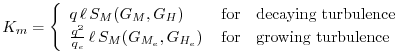
The fizhi package surface Types are designated using the Koster-Suarez (Koster and Suarez [1992,1991]) Land Surface Model (LSM) mosaic philosophy which allows multiple ``tiles'', or multiple surface types, in any one grid cell. The Koster-Suarez LSM surface type classifications are shown in Table 6.16. The surface types and the percent of the grid cell occupied by any surface type were derived from the surface classification of Defries and Townshend [1994], and information about the location of permanent ice was obtained from the classifications of Dorman and Sellers [1989]. The surface type map for a
|
Surface Type Designation
|
6.5.3.2.10 Surface Roughness
The surface roughness length over oceans is computed iteratively with the wind stress by the surface layer parameterization (Helfand and Schubert [1995]). It employs an interpolation between the functions of Large and Pond [1981] for high winds and of Kondo [1975] for weak winds.
6.5.3.2.11 Albedo
The surface albedo computation, described in Koster and Suarez [1991], employs the ``two stream'' approximation used in Sellers' (1987) Simple Biosphere (SiB) Model which distinguishes between the direct and diffuse albedos in the visible and in the near infra-red spectral ranges. The albedos are functions of the observed leaf area index (a description of the relative orientation of the leaves to the sun), the greenness fraction, the vegetation type, and the solar zenith angle. Modifications are made to account for the presence of snow, and its depth relative to the height of the vegetation elements.
6.5.3.2.12 Gravity Wave Drag
The fizhi package employs the gravity wave drag scheme of Zhou et al. [1995]). This scheme is a modified version of Vernekar et al. (1992), which was based on Alpert et al. (1988) and Helfand et al. (1987). In this version, the gravity wave stress at the surface is based on that derived by Pierrehumbert (1986) and is given by:
| (6.38) |
where
![]() is the Froude number,
is the Froude number, ![]() is the Brunt - Väisälä frequency,
is the Brunt - Väisälä frequency, ![]() is the
surface wind speed,
is the
surface wind speed, ![]() is the standard deviation of the sub-grid scale orography,
and
is the standard deviation of the sub-grid scale orography,
and ![]() is the wavelength of the monochromatic gravity wave in the direction of the low-level wind.
A modification introduced by Zhou et al. allows for the momentum flux to
escape through the top of the model, although this effect is small for the current 70-level model.
The subgrid scale standard deviation is defined by
is the wavelength of the monochromatic gravity wave in the direction of the low-level wind.
A modification introduced by Zhou et al. allows for the momentum flux to
escape through the top of the model, although this effect is small for the current 70-level model.
The subgrid scale standard deviation is defined by ![]() , and is not allowed to exceed 400 m.
, and is not allowed to exceed 400 m.
The effects of using this scheme within a GCM are shown in Takacs and Suarez [1996]. Experiments using the gravity wave drag parameterization yielded significant and beneficial impacts on both the time-mean flow and the transient statistics of the a GCM climatology, and have eliminated most of the worst dynamically driven biases in the a GCM simulation. An examination of the angular momentum budget during climate runs indicates that the resulting gravity wave torque is similar to the data-driven torque produced by a data assimilation which was performed without gravity wave drag. It was shown that the inclusion of gravity wave drag results in large changes in both the mean flow and in eddy fluxes. The result is a more accurate simulation of surface stress (through a reduction in the surface wind strength), of mountain torque (through a redistribution of mean sea-level pressure), and of momentum convergence (through a reduction in the flux of westerly momentum by transient flow eddies).
Boundary Conditions and other Input Data:
Required fields which are not explicitly predicted or diagnosed during model execution must either be prescribed internally or obtained from external data sets. In the fizhi package these fields include: sea surface temperature, sea ice estent, surface geopotential variance, vegetation index, and the radiation-related background levels of: ozone, carbon dioxide, and stratospheric moisture.
Boundary condition data sets are available at the model's resolutions for either climatological or yearly varying conditions. Any frequency of boundary condition data can be used in the fizhi package; however, the current selection of data is summarized in Table 6.17. The time mean values are interpolated during each model timestep to the current time.
|
Fizhi Input Datasets
|
6.5.3.2.13 Topography and Topography Variance
Surface geopotential heights are provided from an averaging of the Navy 10 minute by 10 minute dataset supplied by the National Center for Atmospheric Research (NCAR) to the model's grid resolution. The original topography is first rotated to the proper grid-orientation which is being run, and then averages the data to the model resolution.
The standard deviation of the subgrid-scale topography is computed by interpolating the 10 minute data to the model's resolution and re-interpolating back to the 10 minute by 10 minute resolution. The sub-grid scale variance is constructed based on this smoothed dataset.
6.5.3.2.14 Upper Level Moisture
The fizhi package uses climatological water vapor data above 100 mb from the Stratospheric Aerosol and Gas Experiment (SAGE) as input into the model's radiation packages. The SAGE data is archived as monthly zonal means at
6.5.3.3 Fizhi Diagnostics
| NAME | UNITS | LEVELS | DESCRIPTION | |
| UFLUX |
|
1 |
|
|
| VFLUX |
|
1 |
|
|
| HFLUX | 1 |
|
||
| EFLUX | 1 |
|
||
| QICE | 1 |
|
||
| RADLWG | 1 |
|
||
| RADSWG | 1 |
|
||
| RI |
|
Nrphys |
|
|
| CT |
|
1 |
|
|
| CU |
|
1 |
|
|
| ET | Nrphys |
|
||
| EU | Nrphys |
|
||
| TURBU | Nrphys |
|
||
| TURBV | Nrphys |
|
||
| TURBT | Nrphys |
|
||
| TURBQ | Nrphys |
|
||
| MOISTT | Nrphys |
|
||
| MOISTQ | Nrphys |
|
||
| RADLW | Nrphys |
|
||
| RADSW | Nrphys |
|
||
| PREACC | 1 |
|
||
| PRECON | 1 |
|
||
| TUFLUX |
|
Nrphys |
|
|
| TVFLUX |
|
Nrphys |
|
|
| TTFLUX | Nrphys |
|
| NAME | UNITS | LEVELS | DESCRIPTION | |
| TQFLUX | Nrphys |
|
||
| CN |
|
1 |
|
|
| WINDS | 1 |
|
||
| DTSRF | 1 |
|
||
| TG | 1 |
|
||
| TS | 1 |
|
||
| DTG | 1 |
|
||
| QG | 1 |
|
||
| QS | 1 |
|
||
| TGRLW | 1 |
|
||
| ST4 | 1 |
|
||
| OLR | 1 |
|
||
| OLRCLR | 1 |
|
||
| LWGCLR | 1 |
|
||
| LWCLR | Nrphys |
|
||
| TLW | Nrphys |
|
||
| SHLW | Nrphys |
|
||
| OZLW | Nrphys |
|
||
| CLMOLW | Nrphys |
|
||
| CLDTOT | Nrphys |
|
||
| LWGDOWN | 1 |
|
||
| GWDT | Nrphys |
|
||
| RADSWT | 1 |
|
||
| TAUCLD |
|
Nrphys |
|
|
| TAUCLDC | Nrphys |
|
| NAME | UNITS | LEVELS | DESCRIPTION | |
| CLDLOW | Nrphys |
|
||
| EVAP | 1 |
|
||
| DPDT | 1 |
|
||
| UAVE | Nrphys |
|
||
| VAVE | Nrphys |
|
||
| TAVE | Nrphys |
|
||
| QAVE | Nrphys |
|
||
| OMEGA | Nrphys |
|
||
| DUDT | Nrphys |
|
||
| DVDT | Nrphys |
|
||
| DTDT | Nrphys |
|
||
| DQDT | Nrphys |
|
||
| VORT |
|
Nrphys |
|
|
| DTLS | Nrphys |
|
||
| DQLS | Nrphys |
|
||
| USTAR | 1 |
|
||
| Z0 | 1 |
|
||
| FRQTRB | Nrphys-1 |
|
||
| PBL | 1 |
|
||
| SWCLR | Nrphys |
|
||
| OSR | 1 |
|
||
| OSRCLR | 1 |
|
||
| CLDMAS | Nrphys |
|
||
| UAVE | Nrphys |
|
| NAME | UNITS | LEVELS | DESCRIPTION | |
| VAVE | Nrphys |
|
||
| TAVE | Nrphys |
|
||
| QAVE | Nrphys |
|
||
| RFT | Nrphys |
|
||
| PS | 1 |
|
||
| QQAVE | Nrphys |
|
||
| SWGCLR | 1 |
|
||
| PAVE | 1 |
|
||
| DIABU | Nrphys |
|
||
| DIABV | Nrphys |
|
||
| DIABT | Nrphys |
|
||
| DIABQ | Nrphys |
|
||
| RFU | Nrphys |
|
||
| RFV | Nrphys |
|
||
| GWDU | Nrphys |
|
||
| GWDU | Nrphys |
|
||
| GWDUS | 1 |
|
||
| GWDVS | 1 |
|
||
| GWDUT | 1 |
|
||
| GWDVT | 1 |
|
||
| LZRAD | Nrphys |
|
| NAME | UNITS | LEVELS | DESCRIPTION | |
| SLP | 1 |
|
||
| CLDFRC | 1 |
|
||
| TPW | 1 |
|
||
| U2M | 1 |
|
||
| V2M | 1 |
|
||
| T2M | 1 |
|
||
| Q2M | 1 |
|
||
| U10M | 1 |
|
||
| V10M | 1 |
|
||
| T10M | 1 |
|
||
| Q10M | 1 |
|
||
| DTRAIN | Nrphys |
|
||
| QFILL | Nrphys |
|
| NAME | UNITS | LEVELS | DESCRIPTION | |
| DTCONV | Nr |
|
||
| DQCONV | Nr |
|
||
| RELHUM | Nr |
|
||
| PRECLS | 1 |
|
||
| ENPREC | 1 |
|
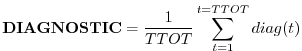
Fizhi Diagnostic Description:
In this section we list and describe the diagnostic quantities available within the GCM. The diagnostics are listed in the order that they appear in the Diagnostic Menu, Section 6.5.3.3. In all cases, each diagnostic as currently archived on the output datasets is time-averaged over its diagnostic output frequency:
where
UFLUX Surface Zonal Wind Stress on the Atmosphere (
![]() )
)
The zonal wind stress is the turbulent flux of zonal momentum from the surface.
where
VFLUX Surface Meridional Wind Stress on the Atmosphere (
![]() )
)
The meridional wind stress is the turbulent flux of meridional momentum from the surface.
where
HFLUX Surface Flux of Sensible Heat (![]() )
)
The turbulent flux of sensible heat from the surface to the atmosphere is a function of the gradient of virtual potential temperature and the eddy exchange coefficient:
where
EFLUX Surface Flux of Latent Heat (![]() )
)
The turbulent flux of latent heat from the surface to the atmosphere is a function of the gradient of moisture, the potential evapotranspiration fraction and the eddy exchange coefficient:
where
QICE Heat Conduction Through Sea Ice (![]() )
)
Over sea ice there is an additional source of energy at the surface due to the heat conduction from the relatively warm ocean through the sea ice. The heat conduction through sea ice represents an additional energy source term for the ground temperature equation.
where ![]() is the thermal conductivity of ice,
is the thermal conductivity of ice, ![]() is the ice thickness, assumed to
be
is the ice thickness, assumed to
be
![]() where sea ice is present,
where sea ice is present, ![]() is 273 degrees Kelvin, and
is 273 degrees Kelvin, and
![]() is the temperature of the sea ice.
is the temperature of the sea ice.
NOTE: QICE is not available through model version 5.3, but is available in subsequent versions.
RADLWG Net upward Longwave Flux at the surface (![]() )
)
where Nrphys+1 indicates the lowest model edge-level, or
RADSWG Net downard shortwave Flux at the surface (![]() )
)
where Nrphys+1 indicates the lowest model edge-level, or
RI Richardson Number (
![]() )
)
The non-dimensional stability indicator is the ratio of the buoyancy to the shear:
where we used the hydrostatic equation:
Negative values indicate unstable buoyancy AND shear, small positive values (
CT Surface Exchange Coefficient for Temperature and Moisture (
![]() )
)
The surface exchange coefficient is obtained from the similarity functions for the stability dependant flux profile relationships:
where
and:
![]() is the similarity function of
is the similarity function of ![]() , which expresses the stability dependance of
the temperature and moisture gradients, specified differently for stable and unstable
layers according to Helfand and Schubert [1995]. k is the Von Karman constant,
, which expresses the stability dependance of
the temperature and moisture gradients, specified differently for stable and unstable
layers according to Helfand and Schubert [1995]. k is the Von Karman constant, ![]() is the
non-dimensional stability parameter, Pr is the Prandtl number for air,
is the
non-dimensional stability parameter, Pr is the Prandtl number for air, ![]() is the molecular
viscosity,
is the molecular
viscosity, ![]() is the surface roughness length,
is the surface roughness length, ![]() is the surface stress velocity
(see diagnostic number 67), and the subscript ref refers to a reference value.
is the surface stress velocity
(see diagnostic number 67), and the subscript ref refers to a reference value.
CU Surface Exchange Coefficient for Momentum (
![]() )
)
The surface exchange coefficient is obtained from the similarity functions for the stability dependant flux profile relationships:
where
ET Diffusivity Coefficient for Temperature and Moisture (![]() )
)
In the level 2.5 version of the Mellor-Yamada (1974) hierarchy, the turbulent heat or
moisture flux for the atmosphere above the surface layer can be expressed as a turbulent
diffusion coefficient ![]() times the negative of the gradient of potential temperature
or moisture. In the Helfand and Labraga [1988] adaptation of this closure,
times the negative of the gradient of potential temperature
or moisture. In the Helfand and Labraga [1988] adaptation of this closure, ![]() takes the form:
takes the form:

where
For the detailed equations and derivations of the modified level 2.5 closure scheme, see Helfand and Labraga [1988].
In the surface layer,
![]() is the exchange coefficient for heat and moisture,
in units of
is the exchange coefficient for heat and moisture,
in units of ![]() , given by:
, given by:
where
EU Diffusivity Coefficient for Momentum (![]() )
)
In the level 2.5 version of the Mellor-Yamada (1974) hierarchy, the turbulent heat
momentum flux for the atmosphere above the surface layer can be expressed as a turbulent
diffusion coefficient ![]() times the negative of the gradient of the u-wind.
In the Helfand and Labraga [1988] adaptation of this closure,
times the negative of the gradient of the u-wind.
In the Helfand and Labraga [1988] adaptation of this closure, ![]() takes the form:
takes the form:

where
For the detailed equations and derivations of the modified level 2.5 closure scheme, see Helfand and Labraga [1988].
In the surface layer,
![]() is the exchange coefficient for momentum,
in units of
is the exchange coefficient for momentum,
in units of ![]() , given by:
, given by:
where
TURBU Zonal U-Momentum changes due to Turbulence (![]() )
)
The tendency of U-Momentum due to turbulence is written:
The Helfand and Labraga level 2.5 scheme models the turbulent
flux of u-momentum in terms of ![]() , and the equation has the form of a diffusion
equation.
, and the equation has the form of a diffusion
equation.
TURBV Meridional V-Momentum changes due to Turbulence (![]() )
)
The tendency of V-Momentum due to turbulence is written:
The Helfand and Labraga level 2.5 scheme models the turbulent
flux of v-momentum in terms of ![]() , and the equation has the form of a diffusion
equation.
, and the equation has the form of a diffusion
equation.
TURBT Temperature changes due to Turbulence (![]() )
)
The tendency of temperature due to turbulence is written:
The Helfand and Labraga level 2.5 scheme models the turbulent
flux of temperature in terms of ![]() , and the equation has the form of a diffusion
equation.
, and the equation has the form of a diffusion
equation.
TURBQ Specific Humidity changes due to Turbulence (![]() )
)
The tendency of specific humidity due to turbulence is written:
The Helfand and Labraga level 2.5 scheme models the turbulent
flux of temperature in terms of ![]() , and the equation has the form of a diffusion
equation.
, and the equation has the form of a diffusion
equation.
MOISTT Temperature Changes Due to Moist Processes (![]() )
)
where:
and
The subscript ![]() refers to convective processes, while the subscript
refers to convective processes, while the subscript ![]() refers to large scale
precipitation processes, or supersaturation rain.
The summation refers to contributions from each cloud type called by RAS.
The dry static energy is given
as
refers to large scale
precipitation processes, or supersaturation rain.
The summation refers to contributions from each cloud type called by RAS.
The dry static energy is given
as ![]() , the convective cloud base mass flux is given as
, the convective cloud base mass flux is given as ![]() , and the cloud entrainment is
given as
, and the cloud entrainment is
given as ![]() , which are explicitly defined in Section 6.5.3.2,
the description of the convective parameterization. The fractional adjustment, or relaxation
parameter, for each cloud type is given as
, which are explicitly defined in Section 6.5.3.2,
the description of the convective parameterization. The fractional adjustment, or relaxation
parameter, for each cloud type is given as ![]() , while
, while
![]() is the rain re-evaporation adjustment.
is the rain re-evaporation adjustment.
MOISTQ Specific Humidity Changes Due to Moist Processes (![]() )
)
where:
and
The subscript
RADLW Heating Rate due to Longwave Radiation (![]() )
)
The net longwave heating rate is calculated as the vertical divergence of the
net terrestrial radiative fluxes.
Both the clear-sky and cloudy-sky longwave fluxes are computed within the
longwave routine.
The subroutine calculates the clear-sky flux,
![]() , first.
For a given cloud fraction,
the clear line-of-sight probability
, first.
For a given cloud fraction,
the clear line-of-sight probability
![]() is computed from the current level pressure
is computed from the current level pressure ![]() to the model top pressure,
to the model top pressure,
![]() , and the model surface pressure,
, and the model surface pressure,
![]() ,
for the upward and downward radiative fluxes.
(see Section 6.5.3.2).
The cloudy-sky flux is then obtained as:
,
for the upward and downward radiative fluxes.
(see Section 6.5.3.2).
The cloudy-sky flux is then obtained as:
Finally, the net longwave heating rate is calculated as the vertical divergence of the net terrestrial radiative fluxes:
or
where ![]() is the accelation due to gravity,
is the accelation due to gravity,
![]() is the heat capacity of air at constant pressure,
and
is the heat capacity of air at constant pressure,
and
RADSW Heating Rate due to Shortwave Radiation (![]() )
)
The net Shortwave heating rate is calculated as the vertical divergence of the net solar radiative fluxes. The clear-sky and cloudy-sky shortwave fluxes are calculated separately. For the clear-sky case, the shortwave fluxes and heating rates are computed with both CLMO (maximum overlap cloud fraction) and CLRO (random overlap cloud fraction) set to zero (see Section 6.5.3.2). The shortwave routine is then called a second time, for the cloudy-sky case, with the true time-averaged cloud fractions CLMO and CLRO being used. In all cases, a normalized incident shortwave flux is used as input at the top of the atmosphere.
The heating rate due to Shortwave Radiation under cloudy skies is defined as:
or
where ![]() is the accelation due to gravity,
is the accelation due to gravity,
![]() is the heat capacity of air at constant pressure, RADSWT is the true incident
shortwave radiation at the top of the atmosphere (See Diagnostic #48), and
is the heat capacity of air at constant pressure, RADSWT is the true incident
shortwave radiation at the top of the atmosphere (See Diagnostic #48), and
PREACC Total (Large-scale + Convective) Accumulated Precipition (![]() )
)
For a change in specific humidity due to moist processes,
![]() ,
the vertical integral or total precipitable amount is given by:
,
the vertical integral or total precipitable amount is given by:
A precipitation rate is defined as the vertically integrated moisture adjustment per Moist Processes
time step, scaled to ![]() .
.
PRECON Convective Precipition (![]() )
)
For a change in specific humidity due to sub-grid scale cumulus convective processes,
![]() ,
the vertical integral or total precipitable amount is given by:
,
the vertical integral or total precipitable amount is given by:
A precipitation rate is defined as the vertically integrated moisture adjustment per Moist Processes
time step, scaled to ![]() .
.
TUFLUX Turbulent Flux of U-Momentum (
![]() )
)
The turbulent flux of u-momentum is calculated for
![]() from the eddy coefficient for momentum:
from the eddy coefficient for momentum:
where ![]() is the air density, and
is the air density, and ![]() is the eddy coefficient.
is the eddy coefficient.
TVFLUX Turbulent Flux of V-Momentum (
![]() )
)
The turbulent flux of v-momentum is calculated for
![]() from the eddy coefficient for momentum:
from the eddy coefficient for momentum:
where ![]() is the air density, and
is the air density, and ![]() is the eddy coefficient.
is the eddy coefficient.
TTFLUX Turbulent Flux of Sensible Heat (![]() )
)
The turbulent flux of sensible heat is calculated for
![]() from the eddy coefficient for heat and moisture:
from the eddy coefficient for heat and moisture:
where ![]() is the air density, and
is the air density, and ![]() is the eddy coefficient.
is the eddy coefficient.
TQFLUX Turbulent Flux of Latent Heat (![]() )
)
The turbulent flux of latent heat is calculated for
![]() from the eddy coefficient for heat and moisture:
from the eddy coefficient for heat and moisture:
where ![]() is the air density, and
is the air density, and ![]() is the eddy coefficient.
is the eddy coefficient.
CN Neutral Drag Coefficient (
![]() )
)
The drag coefficient for momentum obtained by assuming a neutrally stable surface layer:
where ![]() is the Von Karman constant,
is the Von Karman constant, ![]() is the height of the surface layer, and
is the height of the surface layer, and
![]() is the surface roughness.
is the surface roughness.
NOTE: CN is not available through model version 5.3, but is available in subsequent
versions.
WINDS Surface Wind Speed (![]() )
)
The surface wind speed is calculated for the last internal turbulence time step:
where the subscript ![]() refers to the lowest model level.
refers to the lowest model level.
DTSRF Air/Surface Virtual Temperature Difference (
![]() )
)
The air/surface virtual temperature difference measures the stability of the surface layer:
where
![]() is the surface potential evapotranspiration coefficient (
is the surface potential evapotranspiration coefficient (![]() over oceans),
over oceans),
![]() is the saturation specific humidity at the ground temperature
and surface pressure, level
is the saturation specific humidity at the ground temperature
and surface pressure, level ![]() refers to the lowest model level and level
refers to the lowest model level and level ![]() refers to the surface.
refers to the surface.
TG Ground Temperature (
![]() )
)
The ground temperature equation is solved as part of the turbulence package using a backward implicit time differencing scheme:
where ![]() is the net surface downward shortwave radiative flux,
is the net surface downward shortwave radiative flux, ![]() is the
net surface upward longwave radiative flux,
is the
net surface upward longwave radiative flux, ![]() is the heat conduction through
sea ice,
is the heat conduction through
sea ice, ![]() is the upward sensible heat flux,
is the upward sensible heat flux, ![]() is the upward latent heat
flux, and
is the upward latent heat
flux, and ![]() is the total heat capacity of the ground.
is the total heat capacity of the ground.
![]() is obtained by solving a heat diffusion equation
for the penetration of the diurnal cycle into the ground (Blackadar [1977]), and is given by:
is obtained by solving a heat diffusion equation
for the penetration of the diurnal cycle into the ground (Blackadar [1977]), and is given by:
Here, the thermal conductivity,
TS Surface Temperature (
![]() )
)
The surface temperature estimate is made by assuming that the model's lowest
layer is well-mixed, and therefore that ![]() is constant in that layer.
The surface temperature is therefore:
is constant in that layer.
The surface temperature is therefore:
DTG Surface Temperature Adjustment (
![]() )
)
The change in surface temperature from one turbulence time step to the next, solved using the Ground Temperature Equation (see diagnostic number 30) is calculated:
where superscript ![]() refers to the new, updated time level, and the superscript
refers to the new, updated time level, and the superscript ![]() refers to the value at the previous turbulence time level.
refers to the value at the previous turbulence time level.
QG Ground Specific Humidity (![]() )
)
The ground specific humidity is obtained by interpolating between the specific humidity at the lowest model level and the specific humidity of a saturated ground. The interpolation is performed using the potential evapotranspiration function:
where ![]() is the surface potential evapotranspiration coefficient (
is the surface potential evapotranspiration coefficient (![]() over oceans),
and
over oceans),
and
![]() is the saturation specific humidity at the ground temperature and surface
pressure.
is the saturation specific humidity at the ground temperature and surface
pressure.
QS Saturation Surface Specific Humidity (![]() )
)
The surface saturation specific humidity is the saturation specific humidity at the ground temprature and surface pressure:
TGRLW Instantaneous ground temperature used as input to the Longwave radiation subroutine (deg)
where
ST4 Upward Longwave flux at the surface (![]() )
)
where
OLR Net upward Longwave flux at ![]() (
(![]() )
)
where top indicates the top of the first model layer. In the GCM,
OLRCLR Net upward clearsky Longwave flux at ![]() (
(![]() )
)
where top indicates the top of the first model layer. In the GCM,
LWGCLR Net upward clearsky Longwave flux at the surface (![]() )
)
where Nrphys+1 indicates the lowest model edge-level, or
LWCLR Heating Rate due to Clearsky Longwave Radiation (![]() )
)
The net longwave heating rate is calculated as the vertical divergence of the
net terrestrial radiative fluxes.
Both the clear-sky and cloudy-sky longwave fluxes are computed within the
longwave routine.
The subroutine calculates the clear-sky flux,
![]() , first.
For a given cloud fraction,
the clear line-of-sight probability
, first.
For a given cloud fraction,
the clear line-of-sight probability
![]() is computed from the current level pressure
is computed from the current level pressure ![]() to the model top pressure,
to the model top pressure,
![]() , and the model surface pressure,
, and the model surface pressure,
![]() ,
for the upward and downward radiative fluxes.
(see Section 6.5.3.2).
The cloudy-sky flux is then obtained as:
,
for the upward and downward radiative fluxes.
(see Section 6.5.3.2).
The cloudy-sky flux is then obtained as:
Thus, LWCLR is defined as the net longwave heating rate due to the vertical divergence of the clear-sky longwave radiative flux:
or
where ![]() is the accelation due to gravity,
is the accelation due to gravity,
![]() is the heat capacity of air at constant pressure,
and
is the heat capacity of air at constant pressure,
and
TLW Instantaneous temperature used as input to the Longwave radiation subroutine (deg)
where
SHLW Instantaneous specific humidity used as input to the Longwave radiation subroutine (kg/kg)
where
OZLW Instantaneous ozone used as input to the Longwave radiation subroutine (kg/kg)
where
CLMOLW Maximum Overlap cloud fraction used in LW Radiation (![]() )
)
CLMOLW is the time-averaged maximum overlap cloud fraction that has been filled by the Relaxed Arakawa/Schubert Convection scheme and will be used in the Longwave Radiation algorithm. These are convective clouds whose radiative characteristics are assumed to be correlated in the vertical. For a complete description of cloud/radiative interactions, see Section 6.5.3.2.
CLDTOT Total cloud fraction used in LW and SW Radiation (![]() )
)
CLDTOT is the time-averaged total cloud fraction that has been filled by the Relaxed Arakawa/Schubert and Large-scale Convection schemes and will be used in the Longwave and Shortwave Radiation packages. For a complete description of cloud/radiative interactions, see Section 6.5.3.2.
where
CLMOSW Maximum Overlap cloud fraction used in SW Radiation (![]() )
)
CLMOSW is the time-averaged maximum overlap cloud fraction that has been filled by the Relaxed Arakawa/Schubert Convection scheme and will be used in the Shortwave Radiation algorithm. These are convective clouds whose radiative characteristics are assumed to be correlated in the vertical. For a complete description of cloud/radiative interactions, see Section 6.5.3.2.
CLROSW Random Overlap cloud fraction used in SW Radiation (![]() )
)
CLROSW is the time-averaged random overlap cloud fraction that has been filled by the Relaxed Arakawa/Schubert and Large-scale Convection schemes and will be used in the Shortwave Radiation algorithm. These are convective and large-scale clouds whose radiative characteristics are not assumed to be correlated in the vertical. For a complete description of cloud/radiative interactions, see Section 6.5.3.2.
RADSWT Incident Shortwave radiation at the top of the atmosphere (![]() )
)
where
EVAP Surface Evaporation (![]() )
)
The surface evaporation is a function of the gradient of moisture, the potential evapotranspiration fraction and the eddy exchange coefficient:
where
DUDT Total Zonal U-Wind Tendency (![]() )
)
DUDT is the total time-tendency of the Zonal U-Wind due to Hydrodynamic, Diabatic, and Analysis forcing.
DVDT Total Zonal V-Wind Tendency (![]() )
)
DVDT is the total time-tendency of the Meridional V-Wind due to Hydrodynamic, Diabatic, and Analysis forcing.
DTDT Total Temperature Tendency (![]() )
)
DTDT is the total time-tendency of Temperature due to Hydrodynamic, Diabatic,
and Analysis forcing.
DQDT Total Specific Humidity Tendency (![]() )
)
DQDT is the total time-tendency of Specific Humidity due to Hydrodynamic, Diabatic, and Analysis forcing.
USTAR Surface-Stress Velocity (![]() )
)
The surface stress velocity, or the friction velocity, is the wind speed at the surface layer top impeded by the surface drag:
![]() is the non-dimensional surface drag coefficient (see diagnostic
number 10), and
is the non-dimensional surface drag coefficient (see diagnostic
number 10), and ![]() is the surface wind speed (see diagnostic number 28).
is the surface wind speed (see diagnostic number 28).
Z0 Surface Roughness Length (![]() )
)
Over the land surface, the surface roughness length is interpolated to the local
time from the monthly mean data of Dorman and Sellers [1989]. Over the ocean,
the roughness length is a function of the surface-stress velocity, ![]() .
.
where the constants are chosen to interpolate between the reciprocal relation of
Kondo [1975] for weak winds, and the piecewise linear relation of Large and Pond [1981]
for moderate to large winds.
FRQTRB Frequency of Turbulence (![]() )
)
The fraction of time when turbulence is present is defined as the fraction of
time when the turbulent kinetic energy exceeds some minimum value, defined here
to be
![]() . When this criterion is met, a counter is
incremented. The fraction over the averaging interval is reported.
. When this criterion is met, a counter is
incremented. The fraction over the averaging interval is reported.
PBL Planetary Boundary Layer Depth (![]() )
)
The depth of the PBL is defined by the turbulence parameterization to be the depth at which the turbulent kinetic energy reduces to ten percent of its surface value.
where ![]() is the pressure in
is the pressure in ![]() at which the turbulent kinetic energy
reaches one tenth of its surface value, and
at which the turbulent kinetic energy
reaches one tenth of its surface value, and ![]() is the surface pressure.
is the surface pressure.
SWCLR Clear sky Heating Rate due to Shortwave Radiation (![]() )
)
The net Shortwave heating rate is calculated as the vertical divergence of the net solar radiative fluxes. The clear-sky and cloudy-sky shortwave fluxes are calculated separately. For the clear-sky case, the shortwave fluxes and heating rates are computed with both CLMO (maximum overlap cloud fraction) and CLRO (random overlap cloud fraction) set to zero (see Section 6.5.3.2). The shortwave routine is then called a second time, for the cloudy-sky case, with the true time-averaged cloud fractions CLMO and CLRO being used. In all cases, a normalized incident shortwave flux is used as input at the top of the atmosphere.
The heating rate due to Shortwave Radiation under clear skies is defined as:
or
where ![]() is the accelation due to gravity,
is the accelation due to gravity,
![]() is the heat capacity of air at constant pressure, RADSWT is the true incident
shortwave radiation at the top of the atmosphere (See Diagnostic #48), and
is the heat capacity of air at constant pressure, RADSWT is the true incident
shortwave radiation at the top of the atmosphere (See Diagnostic #48), and
OSR Net upward Shortwave flux at the top of the model (![]() )
)
where top indicates the top of the first model layer used in the shortwave radiation routine. In the GCM,
OSRCLR Net upward clearsky Shortwave flux at the top of the model (![]() )
)
where top indicates the top of the first model layer used in the shortwave radiation routine. In the GCM,
CLDMAS Convective Cloud Mass Flux (![]() )
)
The amount of cloud mass moved per RAS timestep from all convective clouds is written:
where
UAVE Time-Averaged Zonal U-Wind (![]() )
)
The diagnostic UAVE is simply the time-averaged Zonal U-Wind over the NUAVE output frequency. This is contrasted to the instantaneous Zonal U-Wind which is archived on the Prognostic Output data stream.
Note, UAVE is computed and stored on the staggered C-grid.
VAVE Time-Averaged Meridional V-Wind (![]() )
)
The diagnostic VAVE is simply the time-averaged Meridional V-Wind over the NVAVE output frequency. This is contrasted to the instantaneous Meridional V-Wind which is archived on the Prognostic Output data stream.
Note, VAVE is computed and stored on the staggered C-grid.
TAVE Time-Averaged Temperature (![]() )
)
The diagnostic TAVE is simply the time-averaged Temperature over the NTAVE output frequency. This is contrasted to the instantaneous Temperature which is archived on the Prognostic Output data stream.
QAVE Time-Averaged Specific Humidity (![]() )
)
The diagnostic QAVE is simply the time-averaged Specific Humidity over the NQAVE output frequency. This is contrasted to the instantaneous Specific Humidity which is archived on the Prognostic Output data stream.
PAVE Time-Averaged Surface Pressure - PTOP (![]() )
)
The diagnostic PAVE is simply the time-averaged Surface Pressure - PTOP over
the NPAVE output frequency. This is contrasted to the instantaneous
Surface Pressure - PTOP which is archived on the Prognostic Output data stream.
QQAVE Time-Averaged Turbulent Kinetic Energy ![]()
The diagnostic QQAVE is simply the time-averaged prognostic Turbulent Kinetic Energy produced by the GCM Turbulence parameterization over the NQQAVE output frequency. This is contrasted to the instantaneous Turbulent Kinetic Energy which is archived on the Prognostic Output data stream.
Note, QQAVE is computed and stored at the ``mass-point'' locations on the staggered C-grid.
SWGCLR Net downward clearsky Shortwave flux at the surface (![]() )
)
where Nrphys+1 indicates the lowest model edge-level, or
DIABU Total Diabatic Zonal U-Wind Tendency (![]() )
)
DIABU is the total time-tendency of the Zonal U-Wind due to Diabatic processes and the Analysis forcing.
DIABV Total Diabatic Meridional V-Wind Tendency (![]() )
)
DIABV is the total time-tendency of the Meridional V-Wind due to Diabatic processes and the Analysis forcing.
DIABT Total Diabatic Temperature Tendency (![]() )
)
DIABT is the total time-tendency of Temperature due to Diabatic processes
and the Analysis forcing.
If we define the time-tendency of Temperature due to Diabatic processes as
then, since there are no surface pressure changes due to Diabatic processes, we may write
where
DIABQ Total Diabatic Specific Humidity Tendency (![]() )
)
DIABQ is the total time-tendency of Specific Humidity due to Diabatic processes and the Analysis forcing.
If we define the time-tendency of Specific Humidity due to Diabatic processes as
then, since there are no surface pressure changes due to Diabatic processes, we may write
Thus, DIABQ may be written as
VINTUQ Vertically Integrated Moisture Flux (
![]() )
)
The vertically integrated moisture flux due to the zonal u-wind is obtained by integrating
![]() over the depth of the atmosphere at each model timestep,
and dividing by the total mass of the column.
over the depth of the atmosphere at each model timestep,
and dividing by the total mass of the column.
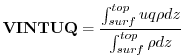
Using
VINTVQ Vertically Integrated Moisture Flux (
![]() )
)
The vertically integrated moisture flux due to the meridional v-wind is obtained by integrating
![]() over the depth of the atmosphere at each model timestep,
and dividing by the total mass of the column.
over the depth of the atmosphere at each model timestep,
and dividing by the total mass of the column.
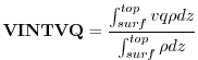
Using
VINTUT Vertically Integrated Heat Flux (
![]() )
)
The vertically integrated heat flux due to the zonal u-wind is obtained by integrating
![]() over the depth of the atmosphere at each model timestep,
and dividing by the total mass of the column.
over the depth of the atmosphere at each model timestep,
and dividing by the total mass of the column.
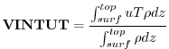
Or,
VINTVT Vertically Integrated Heat Flux (
![]() )
)
The vertically integrated heat flux due to the meridional v-wind is obtained by integrating
![]() over the depth of the atmosphere at each model timestep,
and dividing by the total mass of the column.
over the depth of the atmosphere at each model timestep,
and dividing by the total mass of the column.
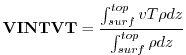
Using
CLDFRC Total 2-Dimensional Cloud Fracton (![]() )
)
If we define the time-averaged random and maximum overlapped cloudiness as CLRO and CLMO respectively, then the probability of clear sky associated with random overlapped clouds at any level is (1-CLRO) while the probability of clear sky associated with maximum overlapped clouds at any level is (1-CLMO). The total clear sky probability is given by (1-CLRO)*(1-CLMO), thus the total cloud fraction at each level may be obtained by 1-(1-CLRO)*(1-CLMO).
At any given level, we may define the clear line-of-site probability by
appropriately accounting for the maximum and random overlap
cloudiness. The clear line-of-site probability is defined to be
equal to the product of the clear line-of-site probabilities
associated with random and maximum overlap cloudiness. The clear
line-of-site probability
![]() associated with maximum overlap clouds,
from the current pressure
associated with maximum overlap clouds,
from the current pressure ![]() to the model top pressure,
to the model top pressure,
![]() , or the model surface pressure,
, or the model surface pressure,
![]() ,
is simply 1.0 minus the largest maximum overlap cloud value along the
line-of-site, ie.
,
is simply 1.0 minus the largest maximum overlap cloud value along the
line-of-site, ie.
Thus, even in the time-averaged sense it is assumed that the maximum overlap clouds are correlated in the vertical. The clear line-of-site probability associated with random overlap clouds is defined to be the product of the clear sky probabilities at each level along the line-of-site, ie.
The total cloud fraction at a given level associated with a line- of-site calculation is given by
![$\displaystyle 1-\left( 1-MAX_p^{p^{\prime}} \left[ CLMO_p \right] \right)
\prod_p^{p^{\prime}} \left( 1-CLRO_p \right)$](img2591.png)
The 2-dimensional net cloud fraction as seen from the top of the atmosphere is given by
![$\displaystyle {\bf CLDFRC} = 1-\left( 1-MAX_{l=l_1}^{Nrphys} \left[ CLMO_l \right] \right)
\prod_{l=l_1}^{Nrphys} \left( 1-CLRO_l \right)
$](img2592.png)
For a complete description of cloud/radiative interactions, see Section 6.5.3.2.
QINT Total Precipitable Water (![]() )
)
The Total Precipitable Water is defined as the vertical integral of the specific humidity,
given by:
where we have used the hydrostatic relation
U2M Zonal U-Wind at 2 Meter Depth (![]() )
)
The u-wind at the 2-meter depth is determined from the similarity theory:
where
![]() is the non-dimensional wind shear at two meters, and the subscript
is the non-dimensional wind shear at two meters, and the subscript
![]() refers to the height of the top of the surface layer. If the roughness height
is above two meters,
refers to the height of the top of the surface layer. If the roughness height
is above two meters, ![]() is undefined.
is undefined.
V2M Meridional V-Wind at 2 Meter Depth (![]() )
)
The v-wind at the 2-meter depth is a determined from the similarity theory:
where
![]() is the non-dimensional wind shear at two meters, and the subscript
is the non-dimensional wind shear at two meters, and the subscript
![]() refers to the height of the top of the surface layer. If the roughness height
is above two meters,
refers to the height of the top of the surface layer. If the roughness height
is above two meters, ![]() is undefined.
is undefined.
T2M Temperature at 2 Meter Depth (
![]() )
)
The temperature at the 2-meter depth is a determined from the similarity theory:
where:
where
![]() is the non-dimensional temperature gradient at two meters,
is the non-dimensional temperature gradient at two meters, ![]() is
the non-dimensional temperature gradient in the viscous sublayer, and the subscript
is
the non-dimensional temperature gradient in the viscous sublayer, and the subscript
![]() refers to the height of the top of the surface layer. If the roughness height
is above two meters,
refers to the height of the top of the surface layer. If the roughness height
is above two meters, ![]() is undefined.
is undefined.
Q2M Specific Humidity at 2 Meter Depth (![]() )
)
The specific humidity at the 2-meter depth is determined from the similarity theory:
where:
where
![]() is the non-dimensional temperature gradient at two meters,
is the non-dimensional temperature gradient at two meters, ![]() is
the non-dimensional temperature gradient in the viscous sublayer, and the subscript
is
the non-dimensional temperature gradient in the viscous sublayer, and the subscript
![]() refers to the height of the top of the surface layer. If the roughness height
is above two meters,
refers to the height of the top of the surface layer. If the roughness height
is above two meters, ![]() is undefined.
is undefined.
U10M Zonal U-Wind at 10 Meter Depth (![]() )
)
The u-wind at the 10-meter depth is an interpolation between the surface wind and the model lowest level wind using the ratio of the non-dimensional wind shear at the two levels:
where
![]() is the non-dimensional wind shear at ten meters, and the subscript
is the non-dimensional wind shear at ten meters, and the subscript
![]() refers to the height of the top of the surface layer.
refers to the height of the top of the surface layer.
V10M Meridional V-Wind at 10 Meter Depth (![]() )
)
The v-wind at the 10-meter depth is an interpolation between the surface wind and the model lowest level wind using the ratio of the non-dimensional wind shear at the two levels:
where
![]() is the non-dimensional wind shear at ten meters, and the subscript
is the non-dimensional wind shear at ten meters, and the subscript
![]() refers to the height of the top of the surface layer.
refers to the height of the top of the surface layer.
T10M Temperature at 10 Meter Depth (
![]() )
)
The temperature at the 10-meter depth is an interpolation between the surface potential temperature and the model lowest level potential temperature using the ratio of the non-dimensional temperature gradient at the two levels:
where:
where
![]() is the non-dimensional temperature gradient at two meters,
is the non-dimensional temperature gradient at two meters, ![]() is
the non-dimensional temperature gradient in the viscous sublayer, and the subscript
is
the non-dimensional temperature gradient in the viscous sublayer, and the subscript
![]() refers to the height of the top of the surface layer.
refers to the height of the top of the surface layer.
Q10M Specific Humidity at 10 Meter Depth (![]() )
)
The specific humidity at the 10-meter depth is an interpolation between the surface specific humidity and the model lowest level specific humidity using the ratio of the non-dimensional temperature gradient at the two levels:
where:
where
![]() is the non-dimensional temperature gradient at two meters,
is the non-dimensional temperature gradient at two meters, ![]() is
the non-dimensional temperature gradient in the viscous sublayer, and the subscript
is
the non-dimensional temperature gradient in the viscous sublayer, and the subscript
![]() refers to the height of the top of the surface layer.
refers to the height of the top of the surface layer.
DTRAIN Cloud Detrainment Mass Flux (![]() )
)
The amount of cloud mass moved per RAS timestep at the cloud detrainment level is written:
where
QFILL Filling of negative Specific Humidity (![]() )
)
Due to computational errors associated with the numerical scheme used for the advection of moisture, negative values of specific humidity may be generated. The specific humidity is checked for negative values after every dynamics timestep. If negative values have been produced, a filling algorithm is invoked which redistributes moisture from below. Diagnostic QFILL is equal to the net filling needed to eliminate negative specific humidity, scaled to a per-day rate:
where
6.5.3.4 Key subroutines, parameters and files
6.5.3.5 Dos and donts
6.5.3.6 Fizhi Reference
6.5.3.7 Experiments and tutorials that use fizhi
- Global atmosphere experiment with realistic SST and topography in fizhi-cs-32x32x10 verification directory.
- Global atmosphere aqua planet experiment in fizhi-cs-aqualev20 verification directory.
Next: 6.6 Sea Ice Packages Up: 6.5 Atmosphere Packages Previous: 6.5.2 Land package Contents mitgcm-support@mitgcm.org
| Copyright © 2006 Massachusetts Institute of Technology | Last update 2018-01-23 |


