Home Contact Us Site Map  
 
       
    next up previous contents
Next: 7.7.3 Key routines Up: 7.7 Potential vorticity Matlab Previous: 7.7.1 Introduction   Contents

Subsections

7.7.2 Equations
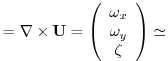
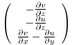
7.7.2.1 Potential Vorticity

The package computes the three components of the relative vorticity defined by:
$\displaystyle \omega$ $\displaystyle = \nabla \times {\bf U} = \left( \begin{array}{c}
\omega_x\\
\omega_y\\
\zeta
\end{array}\right)
\simeq$ $\displaystyle \left( \begin{array}{c}
-\frac{\partial v}{\partial z}\\
-\fr...
...rac{\partial v}{\partial x} - \frac{\partial u}{\partial y}
\end{array}\right)$ (7.1)

where we omitted (like all across the package) the vertical velocity component.

The package then computes the potential vorticity as:

$\displaystyle Q$ $\displaystyle =$ $\displaystyle -\frac{1}{\rho} \omega\cdot\nabla\sigma_\theta$ (7.2)
$\displaystyle Q$ $\displaystyle =$ $\displaystyle -\frac{1}{\rho}\left(\omega_x \frac{\partial \sigma_\theta}{\part...
...ial y} +
\left(f+\zeta\right) \frac{\partial \sigma_\theta}{\partial z}\right)$ (7.3)

where $ \rho $ is the density, $ \sigma_\theta$ is the potential density (both eventually computed by the package) and $ f$ is the Coriolis parameter.

The package is also able to compute the simpler planetary vorticity as:

$\displaystyle splQ$ $\displaystyle =$ $\displaystyle -\frac{f}{\rho}\frac{\sigma_\theta}{\partial z}$ (7.4)

7.7.2.2 Surface vertical potential vorticity fluxes

These quantities are useful in mode water studies because of the impermeability theorem which states that for a given potential density layer (embedding a mode water), the integrated PV only changes through surface input/output.

Vertical PV fluxes due to frictional and diabatic processes are given by:

$\displaystyle J^B_z$ $\displaystyle =$ $\displaystyle -\frac{f}{h}\left( \frac{\alpha Q_{net}}{C_w}-\rho_0 \beta S_{net}\right)$ (7.5)
$\displaystyle J^F_z$ $\displaystyle =$ $\displaystyle \frac{1}{\rho\delta_e} \vec{k}\times\tau\cdot\nabla\sigma_m$ (7.6)

These components can be computed with the package. Details on the variables definition and the way these fluxes are derived can be found in section 7.7.5.


We now give some simple explanations about these fluxes and how they can reduce the PV level of an oceanic potential density layer.

7.7.2.2.1 Diabatic process

Let's take the PV flux due to surface buoyancy forcing from Eq.7.5 and simplify it as:
$\displaystyle J^B_z$ $\displaystyle \simeq$ $\displaystyle -\frac{\alpha f}{hC_w} Q_{net}$ (7.7)

When the net surface heat flux $ Q_{net}$ is upward i.e. negative and cooling the ocean (buoyancy loss), surface density will increase, triggering mixing which reduces the stratification and then the PV.
$\displaystyle Q_{net}$ $\displaystyle <$ $\displaystyle 0 \,\,\,\hbox{(upward, cooling)}$  
$\displaystyle J^B_z$ $\displaystyle >$ $\displaystyle 0 \,\,\,\hbox{(upward)}$  
$\displaystyle -\rho^{-1}\nabla\cdot J^B_z$ $\displaystyle <$ $\displaystyle 0 \,\,\, \hbox{(PV flux divergence)}$  
$\displaystyle PV$ $\displaystyle \searrow$ $\displaystyle \hbox{where $Q_{net}<0$}$  

7.7.2.2.2 Frictional process: "Down-front" wind-stress

Now let's take the PV flux due to the "wind-driven buoyancy flux" from Eq.7.6 and simplify it as:
$\displaystyle J^F_z$ $\displaystyle =$ $\displaystyle \frac{1}{\rho\delta_e} \left( \tau_x\frac{\partial \sigma}{\partial y} - \tau_y\frac{\partial \sigma}{\partial x} \right)$ (7.8)
$\displaystyle J^F_z$ $\displaystyle \simeq$ $\displaystyle \frac{1}{\rho\delta_e} \tau_x\frac{\partial \sigma}{\partial y}$  

When the wind is blowing from the east above the Gulf Stream (a region of high meridional density gradient), it induces an advection of dense water from the northern side of the GS to the southern side through Ekman currents. Then, it induces a "wind-driven" buoyancy lost and mixing which reduces the stratification and the PV.
$\displaystyle \vec{k}\times\tau\cdot\nabla\sigma$ $\displaystyle >$ $\displaystyle 0 \,\,\, \hbox{(''Down-front'' wind)}$  
$\displaystyle J^F_z$ $\displaystyle >$ $\displaystyle 0 \,\,\,\hbox{(upward)}$  
$\displaystyle -\rho^{-1}\nabla\cdot J^F_z$ $\displaystyle <$ $\displaystyle 0 \,\,\, \hbox{(PV flux divergence)}$  
$\displaystyle PV$ $\displaystyle \searrow$ $\displaystyle \hbox{where $\vec{k}\times\tau\cdot\nabla\sigma>0$}$  

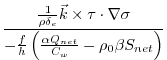
7.7.2.2.3 Diabatic versus frictional processes

A recent debate in the community arose about the relative role of these processes. Taking the ratio of Eq.7.5 and Eq.7.6 leads to:
$\displaystyle \frac{J^F_z}{J^B_Z}$ $\displaystyle =$ $\displaystyle \frac{ \frac{1}{\rho\delta_e} \vec{k}\times\tau\cdot\nabla\sigma }
{-\frac{f}{h}\left( \frac{\alpha Q_{net}}{C_w}-\rho_0 \beta S_{net}\right)}$ (7.9)
  $\displaystyle \simeq$ $\displaystyle \frac{Q_{Ek}/\delta_e}{Q_{net}/h}$  

where appears the lateral heat flux induced by Ekman currents:
$\displaystyle Q_{Ek}$ $\displaystyle =$ $\displaystyle -\frac{C_w}{\alpha\rho f}\vec{k}\times\tau\cdot\nabla\sigma$  
  $\displaystyle =$ $\displaystyle \frac{C_w}{\alpha}\delta_e\vec{u_{Ek}}\cdot\nabla\sigma$ (7.10)

which can be computed with the package. In the aim of comparing both processes, it will be useful to plot surface net and lateral Ekman-induced heat fluxes together with PV fluxes.


next up previous contents
Next: 7.7.3 Key routines Up: 7.7 Potential vorticity Matlab Previous: 7.7.1 Introduction   Contents
mitgcm-support@mitgcm.org
Copyright © 2006 Massachusetts Institute of Technology Last update 2018-01-23