Home Contact Us Site Map  
 
       
    next up previous contents
Next: 2.21.2 Mercator, Nondimensional Equations Up: 2.21 Nonlinear Viscosities for Previous: 2.21 Nonlinear Viscosities for   Contents

Subsections

2.21.1 Eddy Viscosity

A turbulent closure provides an approximation to the 'eddy' terms on the right of the preceding equations. The simplest form of LES is just to increase the viscosity and diffusivity until the viscous and diffusive scales are resolved. That is, we approximate:
$\displaystyle \left({\overline{\frac{D{{\tilde u}}}{Dt} }}-{\frac{\overline{D}{...
...rac{{\frac{\partial^2{{\tilde {\overline{u}}}}}{{\partial{z}}^2}}}{{\rm Re}_v},$   $\displaystyle \left({\overline{\frac{D{{\tilde v}}}{Dt} }}-{\frac{\overline{D}{...
...frac{{\frac{\partial^2{{\tilde {\overline{v}}}}}{{\partial{z}}^2}}}{{\rm Re}_v}$  
$\displaystyle \left(\overline{\frac{D{w}}{Dt}}-\frac{\overline{D}{\overline{w}}...
... Re}_h}
+\frac{{\frac{\partial^2{\overline{w}}}{{\partial{z}}^2}}}{{\rm Re}_v},$   $\displaystyle \left(\overline{\frac{D{b}}{Dt}}-\frac{\overline{D}{\ \overline{b...
...rac{{\frac{\partial^2{\overline{b}}}{{\partial{z}}^2}}}{\Pr{\rm Re}_v}\nonumber$  

2.21.1.1 Reynolds-Number Limited Eddy Viscosity

One way of ensuring that the gridscale is sufficiently viscous (ie. resolved) is to choose the eddy viscosity $ A_h$ so that the gridscale horizontal Reynolds number based on this eddy viscosity, $ {\rm Re}_h$ , to is O(1). That is, if the gridscale is to be viscous, then the viscosity should be chosen to make the viscous terms as large as the advective ones. Bryan et al Bryan et al. [1975] notes that a computational mode is squelched by using $ {\rm Re}_h<$ 2.

MITgcm users can select horizontal eddy viscosities based on $ {\rm Re}_h$ using two methods. 1) The user may estimate the velocity scale expected from the calculation and grid spacing and set the viscAh to satisfy $ {\rm Re}_h<2$ . 2) The user may use viscAhReMax, which ensures that the viscosity is always chosen so that $ {\rm Re}_h<{\sf viscAhReMax}$ . This last option should be used with caution, however, since it effectively implies that viscous terms are fixed in magnitude relative to advective terms. While it may be a useful method for specifying a minimum viscosity with little effort, tests Bryan et al. [1975] have shown that setting viscAhReMax=2 often tends to increase the viscosity substantially over other more 'physical' parameterizations below, especially in regions where gradients of velocity are small (and thus turbulence may be weak), so perhaps a more liberal value should be used, eg. viscAhReMax=10.

While it is certainly necessary that viscosity be active at the gridscale, the wavelength where dissipation of energy or enstrophy occurs is not necessarily $ L=A_h/U$ . In fact, it is by ensuring that the either the dissipation of energy in a 3-d turbulent cascade (Smagorinsky) or dissipation of enstrophy in a 2-d turbulent cascade (Leith) is resolved that these parameterizations derive their physical meaning.

2.21.1.2 Vertical Eddy Viscosities

Vertical eddy viscosities are often chosen in a more subjective way, as model stability is not usually as sensitive to vertical viscosity. Usually the 'observed' value from finescale measurements, etc., is used (eg. viscAr $ \approx1\times10^{-4} m^2/s$ ). However, Smagorinsky Smagorinsky [1993] notes that the Smagorinsky parameterization of isotropic turbulence implies a value of the vertical viscosity as well as the horizontal viscosity (see below).

2.21.1.3 Smagorinsky Viscosity

Some Smagorinsky [1963,1993] suggest choosing a viscosity that depends on the resolved motions. Thus, the overall viscous operator has a nonlinear dependence on velocity. Smagorinsky chose his form of viscosity by considering Kolmogorov's ideas about the energy spectrum of 3-d isotropic turbulence.

Kolmogorov suppposed that is that energy is injected into the flow at large scales (small $ k$ ) and is 'cascaded' or transferred conservatively by nonlinear processes to smaller and smaller scales until it is dissipated near the viscous scale. By setting the energy flux through a particular wavenumber $ k$ , $ \epsilon$ , to be a constant in $ k$ , there is only one combination of viscosity and energy flux that has the units of length, the Kolmogorov wavelength. It is $ L_\epsilon(\nu)\propto\pi\epsilon^{-1/4}\nu^{3/4}$ (the $ \pi$ stems from conversion from wavenumber to wavelength). To ensure that this viscous scale is resolved in a numerical model, the gridscale should be decreased until $ L_\epsilon(\nu)>L$ (so-called Direct Numerical Simulation, or DNS). Alternatively, an eddy viscosity can be used and the corresponding Kolmogorov length can be made larger than the gridscale, $ L_\epsilon(A_h)\propto\pi\epsilon^{-1/4}A_h^{3/4}$ (for Large Eddy Simulation or LES).

There are two methods of ensuring that the Kolmogorov length is resolved in MITgcm. 1) The user can estimate the flux of energy through spectral space for a given simulation and adjust grid spacing or viscAh to ensure that $ L_\epsilon(A_h)>L$ . 2) The user may use the approach of Smagorinsky with viscC2Smag, which estimates the energy flux at every grid point, and adjusts the viscosity accordingly.

Smagorinsky formed the energy equation from the momentum equations by dotting them with velocity. There are some complications when using the hydrostatic approximation as described by Smagorinsky Smagorinsky [1993]. The positive definite energy dissipation by horizontal viscosity in a hydrostatic flow is
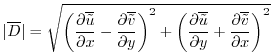
 $ \nu D^2$ , where D is the deformation rate at the viscous scale. According to Kolmogorov's theory, this should be a good approximation to the energy flux at any wavenumber $ \epsilon\approx\nu D^2$ . Kolmogorov and Smagorinsky noted that using an eddy viscosity that exceeds the molecular value $ \nu$ should ensure that the energy flux through viscous scale set by the eddy viscosity is the same as it would have been had we resolved all the way to the true viscous scale. That is, $ \epsilon\approx
A_{hSmag} \overline{D}^2$ . If we use this approximation to estimate the Kolmogorov viscous length, then

$\displaystyle L_\epsilon(A_{hSmag})\propto\pi\epsilon^{-1/4}A_{hSmag}^{3/4}\app...
... \overline{D}^2)^{-1/4}A_{hSmag}^{3/4} = \pi A_{hSmag}^{1/2}\overline{D}^{-1/2}$ (2.208)

To make $ L_\epsilon(A_{hSmag})$ scale with the gridscale, then

$\displaystyle A_{hSmag} = \left(\frac{{\sf viscC2Smag}}{\pi}\right)^2L^2\vert\overline{D}\vert$ (2.209)

Where the deformation rate appropriate for hydrostatic flows with shallow-water scaling is

$\displaystyle \vert\overline{D}\vert=\sqrt{\left({\frac{\partial{\overline{{\ti...
...{\partial{y}}}+{\frac{\partial{\overline{{\tilde v}} }}{\partial{x}}}\right)^2}$ (2.210)

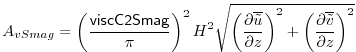
The coefficient viscC2Smag is what an MITgcm user sets, and it replaces the proportionality in the Kolmogorov length with an equality. Others Griffies and Hallberg [2000] suggest values of viscC2Smag from 2.2 to 4 for oceanic problems. Smagorinsky Smagorinsky [1993] shows that values from 0.2 to 0.9 have been used in atmospheric modeling.

Smagorinsky Smagorinsky [1993] shows that a corresponding vertical viscosity should be used:

$\displaystyle A_{vSmag}=\left(\frac{{\sf viscC2Smag}}{\pi}\right)^2H^2 \sqrt{\l...
...ight)^2 +\left({\frac{\partial{\overline{{\tilde v}} }}{\partial{z}}}\right)^2}$ (2.211)

This vertical viscosity is currently not implemented in MITgcm (although it may be soon).

2.21.1.4 Leith Viscosity

Leith Leith [1968,1996] notes that 2-d turbulence is quite different from 3-d. In two-dimensional turbulence, energy cascades to larger scales, so there is no concern about resolving the scales of energy dissipation. Instead, another quantity, enstrophy, (which is the vertical component of vorticity squared) is conserved in 2-d turbulence, and it cascades to smaller scales where it is dissipated.

Following a similar argument to that above about energy flux, the enstrophy flux is estimated to be equal to the positive-definite gridscale dissipation rate of enstrophy $ \eta\approx A_{hLeith}
\vert\nabla\overline{\omega}_3\vert^2$ . By dimensional analysis, the enstrophy-dissipation scale is $ L_\eta(A_{hLeith})\propto\pi
A_{hLeith}^{1/2}\eta^{-1/6}$ . Thus, the Leith-estimated length scale of enstrophy-dissipation and the resulting eddy viscosity are

$\displaystyle L_\eta(A_{hLeith})\propto\pi A_{hLeith}^{1/2}\eta^{-1/6}$ $\displaystyle =$ $\displaystyle \pi A_{hLeith}^{1/3}\vert\nabla \overline{\omega}_3\vert^{-1/3}$ (2.212)
$\displaystyle A_{hLeith}$ $\displaystyle =$ $\displaystyle \left(\frac{{\sf viscC2Leith}}{\pi}\right)^3L^3\vert\nabla \overline{\omega}_3\vert$ (2.213)
$\displaystyle \vert\nabla\omega_3\vert$ $\displaystyle \equiv$ $\displaystyle \sqrt{\left[{\frac{\partial{\ }}{\partial{x}}}
\left({\frac{\par...
...{x}}}
-{\frac{\partial{\overline{{\tilde u}} }}{\partial{y}}}\right)\right]^2}$ (2.214)

2.21.1.5 Modified Leith Viscosity

The argument above for the Leith viscosity parameterization uses concepts from purely 2-dimensional turbulence, where the horizontal flow field is assumed to be divergenceless. However, oceanic flows are only quasi-two dimensional. While the barotropic flow, or the flow within isopycnal layers may behave nearly as two-dimensional turbulence, there is a possibility that these flows will be divergent. In a high-resolution numerical model, these flows may be substantially divergent near the grid scale, and in fact, numerical instabilities exist which are only horizontally divergent and have little vertical vorticity. This causes a difficulty with the Leith viscosity, which can only responds to buildup of vorticity at the grid scale.

MITgcm offers two options for dealing with this problem. 1) The Smagorinsky viscosity can be used instead of Leith, or in conjunction with Leith-a purely divergent flow does cause an increase in Smagorinsky viscosity. 2) The viscC2LeithD parameter can be set. This is a damping specifically targeting purely divergent instabilities near the gridscale. The combined viscosity has the form:

$\displaystyle A_{hLeith}$ $\displaystyle =$ $\displaystyle L^3\sqrt{\left(\frac{{\sf viscC2Leith}}{\pi}\right)^6
\vert\nabl...
...C2LeithD}}{\pi}\right)^6
\vert\nabla \nabla\cdot \overline{\tilde u}_h\vert^2}$ (2.215)
$\displaystyle \vert\nabla \nabla\cdot \overline{\tilde u}_h\vert$ $\displaystyle \equiv$ $\displaystyle \sqrt{\left[{\frac{\partial{\ }}{\partial{x}}}\left({\frac{\parti...
...{x}}}
+{\frac{\partial{\overline{{\tilde v}} }}{\partial{y}}}\right)\right]^2}$ (2.216)

Whether there is any physical rationale for this correction is unclear at the moment, but the numerical consequences are good. The divergence in flows with the grid scale larger or comparable to the Rossby radius is typically much smaller than the vorticity, so this adjustment only rarely adjusts the viscosity if $ {\sf
viscC2LeithD}={\sf viscC2Leith}$ . However, the rare regions where this viscosity acts are often the locations for the largest vales of vertical velocity in the domain. Since the CFL condition on vertical velocity is often what sets the maximum timestep, this viscosity may substantially increase the allowable timestep without severely compromising the verity of the simulation. Tests have shown that in some calculations, a timestep three times larger was allowed when $ {\sf
viscC2LeithD}={\sf viscC2Leith}$ .

2.21.1.6 Courant-Freidrichs-Lewy Constraint on Viscosity

Whatever viscosities are used in the model, the choice is constrained by gridscale and timestep by the Courant-Freidrichs-Lewy (CFL) constraint on stability:
$\displaystyle A_h$ $\displaystyle <$ $\displaystyle \frac{L^2}{4\Delta t}$ (2.217)
$\displaystyle A_4$ $\displaystyle \le$ $\displaystyle \frac{L^4}{32\Delta t}$ (2.218)

The viscosities may be automatically limited to be no greater than these values in MITgcm by specifying viscAhGridMax$ <1$ and viscA4GridMax$ <1$ . Similarly-scaled minimum values of viscosities are provided by viscAhGridMin and viscA4GridMin, which if used, should be set to values $ \ll 1$ . $ L$ is roughly the gridscale (see below).

Following Griffies and Hallberg [2000], we note that there is a factor of $ \Delta
x^2/8$ difference between the harmonic and biharmonic viscosities. Thus, whenever a non-dimensional harmonic coefficient is used in the MITgcm (eg. viscAhGridMax$ <1$ ), the biharmonic equivalent is scaled so that the same non-dimensional value can be used (eg. viscA4GridMax$ <1$ ).

2.21.1.7 Biharmonic Viscosity

Holland [1978] suggested that eddy viscosities ought to be focuses on the dynamics at the grid scale, as larger motions would be 'resolved'. To enhance the scale selectivity of the viscous operator, he suggested a biharmonic eddy viscosity instead of a harmonic (or Laplacian) viscosity:
$\displaystyle \left({\overline{\frac{D{{\tilde u}}}{Dt} }}-{\frac{\overline{D}{...
...rac{{\frac{\partial^2{{\tilde {\overline{u}}}}}{{\partial{z}}^2}}}{{\rm Re}_v},$   $\displaystyle \left({\overline{\frac{D{{\tilde v}}}{Dt} }}-{\frac{\overline{D}{...
...frac{{\frac{\partial^2{{\tilde {\overline{v}}}}}{{\partial{z}}^2}}}{{\rm Re}_v}$  
$\displaystyle \left(\overline{\frac{D{w}}{Dt}}-\frac{\overline{D}{\overline{w}}...
... Re}_h}
+\frac{{\frac{\partial^2{\overline{w}}}{{\partial{z}}^2}}}{{\rm Re}_v},$   $\displaystyle \left(\overline{\frac{D{b}}{Dt}}-\frac{\overline{D}{\ \overline{b...
...rac{{\frac{\partial^2{\overline{b}}}{{\partial{z}}^2}}}{\Pr{\rm Re}_v}\nonumber$  

Griffies and Hallberg [2000] propose that if one scales the biharmonic viscosity by stability considerations, then the biharmonic viscous terms will be similarly active to harmonic viscous terms at the gridscale of the model, but much less active on larger scale motions. Similarly, a biharmonic diffusivity can be used for less diffusive flows.

In practice, biharmonic viscosity and diffusivity allow a less viscous, yet numerically stable, simulation than harmonic viscosity and diffusivity. However, there is no physical rationale for such operators being of leading order, and more boundary conditions must be specified than for the harmonic operators. If one considers the approximations of 2.208 and 2.219 to be terms in the Taylor series expansions of the eddy terms as functions of the large-scale gradient, then one can argue that both harmonic and biharmonic terms would occur in the series, and the only question is the choice of coefficients. Using biharmonic viscosity alone implies that one zeros the first non-vanishing term in the Taylor series, which is unsupported by any fluid theory or observation.

Nonetheless, MITgcm supports a plethora of biharmonic viscosities and diffusivities, which are controlled with parameters named similarly to the harmonic viscosities and diffusivities with the substitution $ h\rightarrow 4$ . MITgcm also supports a biharmonic Leith and Smagorinsky viscosities:

$\displaystyle A_{4Smag}$ $\displaystyle =$ $\displaystyle \left(\frac{{\sf viscC4Smag}}{\pi}\right)^2\frac{L^4}{8}\vert D\vert$ (2.219)
$\displaystyle A_{4Leith}$ $\displaystyle =$ $\displaystyle \frac{L^5}{8}\sqrt{\left(\frac{{\sf viscC4Leith}}{\pi}\right)^6
...
...hD}}{\pi}\right)^6
\vert\nabla \nabla\cdot \overline{\bf {\tilde u}}_h\vert^2}$ (2.220)

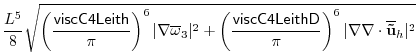
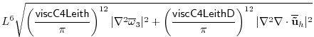
However, it should be noted that unlike the harmonic forms, the biharmonic scaling does not easily relate to whether energy-dissipation or enstrophy-dissipation scales are resolved. If similar arguments are used to estimate these scales and scale them to the gridscale, the resulting biharmonic viscosities should be:
$\displaystyle A_{4Smag}$ $\displaystyle =$ $\displaystyle \left(\frac{{\sf viscC4Smag}}{\pi}\right)^5L^5
\vert\nabla^2\overline{\bf {\tilde u}}_h\vert$ (2.221)
$\displaystyle A_{4Leith}$ $\displaystyle =$ $\displaystyle L^6\sqrt{\left(\frac{{\sf viscC4Leith}}{\pi}\right)^{12}
\vert\n...
...\pi}\right)^{12}
\vert\nabla^2 \nabla\cdot \overline{\bf {\tilde u}}_h\vert^2}$ (2.222)

Thus, the biharmonic scaling suggested by Griffies and Hallberg [2000] implies:
$\displaystyle \vert D\vert$ $\displaystyle \propto$ $\displaystyle L\vert\nabla^2\overline{\bf {\tilde u}}_h\vert$ (2.223)
$\displaystyle \vert\nabla \overline{\omega}_3\vert$ $\displaystyle \propto$ $\displaystyle L\vert\nabla^2 \overline{\omega}_3\vert$ (2.224)

It is not at all clear that these assumptions ought to hold. Only the Griffies and Hallberg [2000] forms are currently implemented in MITgcm.

2.21.1.8 Selection of Length Scale

Above, the length scale of the grid has been denoted $ L$ . However, in strongly anisotropic grids, $ L_x$ and $ L_y$ will be quite different in some locations. In that case, the CFL condition suggests that the minimum of $ L_x$ and $ L_y$ be used. On the other hand, other viscosities which involve whether a particular wavelength is 'resolved' might be better suited to use the maximum of $ L_x$ and $ L_y$ . Currently, MITgcm uses useAreaViscLength to select between two options. If false, the geometric mean of $ L^2_x$ and $ L^2_y$ is used for all viscosities, which is closer to the minimum and occurs naturally in the CFL constraint. If useAreaViscLength is true, then the square root of the area of the grid cell is used.


next up previous contents
Next: 2.21.2 Mercator, Nondimensional Equations Up: 2.21 Nonlinear Viscosities for Previous: 2.21 Nonlinear Viscosities for   Contents
mitgcm-support@mitgcm.org
Copyright © 2006 Massachusetts Institute of Technology Last update 2018-01-23