8.2 PROFILES: model-data comparisons at observed locations

The purpose of pkg/profiles is to allow sampling of MITgcm runs according to a chosen pathway (after a ship or a drifter, along altimeter tracks, etc.), typically leading to easy model-data comparisons. Given input files that contain positions and dates, pkg/profiles will interpolate the model trajectory at the observed location. In particular, pkg/profiles can be used to do model-data comparison online and formulate a least-squares problem (ECCO application).

pkg/profiles is associated with three CPP keys:
(k1) ALLOW_PROFILES
(k2) ALLOW_PROFILES_GENERICGRID
(k3) ALLOW_PROFILES_CONTRIBUTION
k1 switches the package on. By default, pkg/profiles assumes a regular lat-long grid. For other grids such as the cubed sphere, k2 and pre-processing (see below) are necessary. k3 switches the least-squares application on (pkg/ecco needed). pkg/profiles requires needs pkg/cal and netcdf libraries.

The namelist (data.profiles) is illustrated in table 8.7. This example includes two input netcdf files name (ARGOifremer_r8.nc and XBT_v5.nc are to be provided) and cost function multipliers (for least-squares only). The first index is a file number and the second index (in mult* only) is a variable number. By convention, the variable number is an integer ranging 1 to 6: temperature, salinity, zonal velocity, meridional velocity, sea surface height anomaly, and passive tracer.

The input file structure is illustrated in table 8.8. To create such files, one can use the netcdf_ecco_create.m matlab script, which can be checked out of
MITgcm_contrib/gael/profilesMatlabProcessing/
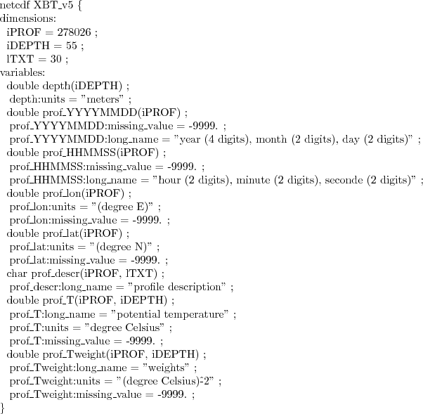
along with a full suite of matlab scripts associated with pkg/profiles. At run time, each file is scanned to determine which variables are included; these will be interpolated. The (final) output file structure is similar but with interpolated model values in prof_T etc., and it contains model mask variables (e.g. prof_Tmask). The very model output consists of one binary (or netcdf) file per processor. The final netcdf output is to be built from those using netcdf_ecco_recompose.m (offline).

When the k2 option is used (e.g. for cubed sphere runs), the input file is to be completed with interpolation grid points and coefficients computed offline using netcdf_ecco_GenericgridMain.m. Typically, you would first provide the standard namelist and files. After detecting that interpolation information is missing, the model will generate special grid files (profilesXCincl1PointOverlap* etc.) and then stop. You then want to run netcdf_ecco_GenericgridMain.m using the special grid files. This operation could eventually be inlined.

**Table 8.7:** pkg/profiles: data.profiles example.
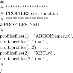$\begin{table}\begin{tabbing} \char93 \\ \char93 ******************\\ \char93 ... ...5',\\ mult\_profiles(2,1) = 1.,\\ \char93 \\ /\\ \end{tabbing} \end{table}$

**Table 8.8:** pkg/profiles: input file structure as would be shown by "ncdump -h ARGOifremer_r8.nc".
$\begin{table}\begin{tabbing} netcdf XBT\_v5 \{\\ dimensions:\\ \hspace{0.1cm} ... ...\> \> prof\_Tweight:missing\_value = -9999. ;\\ \}\\ \end{tabbing} \end{table}$

Last update 2018-01-23