|
|
|
|


Next: 1.3.1 Kinematic Boundary conditions
Up: 1. Overview of MITgcm
Previous: 1.2.9 Simulations of laboratory
Contents
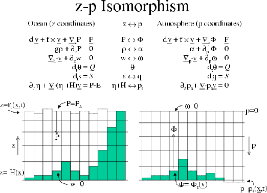
To render atmosphere and ocean models from one dynamical core we exploit
`isomorphisms' between equation sets that govern the evolution of the
respective fluids - see figure 1.14.
One system of hydrodynamical equations is written down
and encoded. The model variables have different interpretations depending on
whether the atmosphere or ocean is being studied. Thus, for example, the
vertical coordinate ` ' is interpreted as pressure,
  , if we are
modeling the atmosphere (right hand side of figure 1.14)
and height,
  , if we are modeling the ocean (left hand side of figure
1.14).
Figure 1.14:
Isomorphic equation sets used for atmosphere (right) and
ocean (left).
|
|
The state of the fluid at any time is characterized by the distribution of
velocity
 , active tracers
  and
and  , a
`geopotential'
  and density
 which may
depend on
  ,
,  , and
, and  . The equations that govern the evolution
of these fields, obtained by applying the laws of classical mechanics and
thermodynamics to a Boussinesq, Navier-Stokes fluid are, written in terms of
a generic vertical coordinate,
  , so that the appropriate
kinematic boundary conditions can be applied isomorphically
see figure 1.15.
Figure 1.15:
Vertical coordinates and kinematic boundary conditions
for atmosphere (top) and ocean (bottom).
|
|
 horizontal mtm horizontal mtm |
(1.1) |
 vertical mtm vertical mtm |
(1.2) |
 continuity continuity |
(1.3) |
 equation of state equation of state |
(1.4) |
 potential temperature potential temperature |
(1.5) |
 humidity/salinity humidity/salinity |
(1.6) |
Here:
 is the vertical coordinate is the vertical coordinate |
|
 is the total derivative is the total derivative |
|
 is the `grad' operator is the `grad' operator |
|
with
 operating in the horizontal and
 operating in the vertical, where
 is a unit vector in the vertical
 is time is time |
|
 is the velocity is the velocity |
|
 is the `pressure'/`geopotential' is the `pressure'/`geopotential' |
|
 is the Earth's rotation is the Earth's rotation |
|
 is the `buoyancy' is the `buoyancy' |
|
 is potential temperature is potential temperature |
|
 is specific humidity in the atmosphere; salinity in the ocean is specific humidity in the atmosphere; salinity in the ocean |
|
 are forcing and dissipation of are forcing and dissipation of  |
|
 are forcing and dissipation of are forcing and dissipation of  |
|
 are forcing and dissipation of are forcing and dissipation of  |
|
The
 and
and
 are provided by
`physics' and forcing packages for atmosphere and ocean. These are described
in later chapters.
Subsections


Next: 1.3.1 Kinematic Boundary conditions
Up: 1. Overview of MITgcm
Previous: 1.2.9 Simulations of laboratory
Contents
mitgcm-support@mitgcm.org
| Copyright © 2006
Massachusetts Institute of Technology |
Last update 2018-01-23 |
 |
|


![\includegraphics[trim=210 80 70 140,width=.9\textwidth, clip]{s_overview/figs/vertcoord.eps}](img118.png)


