3.15.2 Overview

This example experiment demonstrates using the MITgcm to simulate the planetary ocean circulation. The simulation is configured with realistic geography and bathymetry on a $4^{\circ} \times 4^{\circ}$ spherical polar grid. Twenty vertical layers are used in the vertical, ranging in thickness from $50\,{\rm m}$ at the surface to $815\,{\rm m}$ at depth, giving a maximum model depth of $6\,{\rm km}$ . At this resolution, the configuration can be integrated forward for thousands of years on a single processor desktop computer.

The model is forced with climatological wind stress data and surface flux data from Da Silva [10]. Climatological data from Levitus [36] is used to initialize the model hydrography. Levitus data is also used throughout the calculation to derive air-sea fluxes of heat at the ocean surface. These fluxes are combined with climatological estimates of surface heat flux and fresh water, resulting in a mixed boundary condition of the style described in Haney [25]. Altogether, this yields the following forcing applied in the model surface layer.

$\displaystyle {\cal F}_{u}$	$\displaystyle =$	$\displaystyle \frac{\tau_{x}}{\rho_{0} \Delta z_{s}}$	(3.96)
$\displaystyle {\cal F}_{v}$	$\displaystyle =$	$\displaystyle \frac{\tau_{y}}{\rho_{0} \Delta z_{s}}$	(3.97)
$\displaystyle {\cal F}_{\theta}$	$\displaystyle =$	$\displaystyle - \lambda_{\theta} ( \theta - \theta^{\ast} ) - \frac{1}{C_{p} \rho_{0} \Delta z_{s}}{\cal Q}$	(3.98)
$\displaystyle {\cal F}_{s}$	$\displaystyle =$	$\displaystyle - \lambda_{s} ( S - S^{\ast} ) + \frac{S_{0}}{\Delta z_{s}}({\cal E} - {\cal P} - {\cal R})$	(3.99)

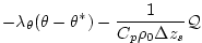
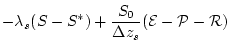
where ${\cal F}_{u}$ , ${\cal F}_{v}$ , ${\cal F}_{\theta}$ , ${\cal F}_{s}$ are the forcing terms in the zonal and meridional momentum and in the potential temperature and salinity equations respectively. The term $\Delta z_{s}$ represents the top ocean layer thickness. It is used in conjunction with the reference density, $\rho_{0}$ (here set to $999.8\,{\rm kg\,m^{-3}}$ ), the reference salinity, $S_{0}$ (here set to 35ppt), and a specific heat capacity $C_{p}$ to convert wind-stress fluxes given in ${\rm N}\,m^{-2}$ ,