Next: 3.8.1 Equations Solved
Up: 3. Getting Started with
Previous: 3.7 Tutorials
Contents
3.8 Barotropic Ocean Gyre In Cartesian Coordinates
This example experiment demonstrates using the MITgcm to simulate
a Barotropic, wind-forced, ocean gyre circulation. The experiment
is a numerical rendition of the gyre circulation problem similar
to the problems described analytically by Stommel in 1966
[49] and numerically in Holland et. al [31].
In this experiment the model
is configured to represent a rectangular enclosed box of fluid,
 km in lateral extent. The fluid is km in lateral extent. The fluid is  km deep and is forced
by a constant in time zonal wind stress, km deep and is forced
by a constant in time zonal wind stress,  , that varies sinusoidally
in the ``north-south'' direction. Topologically the grid is Cartesian and
the coriolis parameter , that varies sinusoidally
in the ``north-south'' direction. Topologically the grid is Cartesian and
the coriolis parameter  is defined according to a mid-latitude beta-plane
equation is defined according to a mid-latitude beta-plane
equation
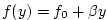 |
(3.1) |
where  is the distance along the ``north-south'' axis of the
simulated domain. For this experiment is the distance along the ``north-south'' axis of the
simulated domain. For this experiment  is set to is set to
 in
(3.1) and in
(3.1) and
 . .
The sinusoidal wind-stress variations are defined according to
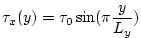 |
(3.2) |
where  is the lateral domain extent ( is the lateral domain extent ( km) and km) and
 is set to is set to
 . .
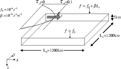
Figure 3.1
summarizes the configuration simulated.
Figure 3.1:
Schematic of simulation domain and wind-stress forcing function
for barotropic gyre numerical experiment. The domain is enclosed bu solid
walls at  0,1200km and at 0,1200km and at  0,1200km. 0,1200km.
 |
Subsections
Next: 3.8.1 Equations Solved
Up: 3. Getting Started with
Previous: 3.7 Tutorials
Contents
mitgcm-support@dev.mitgcm.org
| Copyright © 2002
Massachusetts Institute of Technology |
 |
|