|
|
|
|


Next: 8.1.2 Hydrographic constraints
Up: 8.1 The ECCO state
Previous: 8.1 The ECCO state
Contents
Subsections
Altimetric SSH contributions from T/P and ERS-1/2 are four-fold:
- an
 time mean SSH misfit between
model and T/P time mean SSH misfit between
model and T/P
- daily SSH anomaly misfits between T/P and model
- daily SSH anomaly misfits between ERS-1/2 and model
- daily absolute SSH misfit between T/P and model,
weighted by the full geoid error covariance.
| |
|
|
|
| field |
file name |
deccription |
unit |
| |
|
|
|
| |
|
|
|
| psbar |
psbarfile |
daily model mean SSH fields |
[m] |
| tpmean |
topexmeanfile |
T/P mean |
[cm] |
| tpobs |
topexfile |
daily T/P SSH anomalies |
[cm] |
| erspobs |
ersfile |
daily ERS-1/2 SSH anomalies |
[cm] |
| wp |
geoid_errfile |
diagonal of geoid error covariance |
[m] |
| wtp, wers |
ssh_errfile |
rms of SSH anomalies |
[cm] |
| |
|
|
|
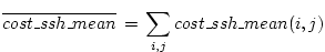
- Compute model mean spatial distribution
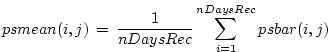 |
(8.1) |
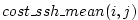
- Compute global offset between model and T/P mean:
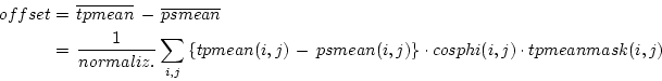 |
(8.2) |
- Misfits are computed w.r.t. global
 . .
First spatial distribution:
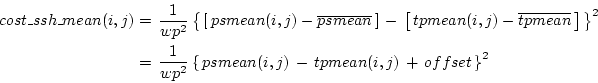 |
(8.3) |
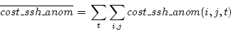
Finally, sum over all spatial entries:
 |
(8.4) |
Computation is same for T/P and ERS-1/2.
Here we write out computation for T/P.
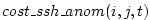
- Compute difference in anomalies:
![\begin{displaymath}\begin{split}cost\_ssh\_anom(i,j,t) & = \, \frac{1}{wtp^2} \l...
... \, \left[ \, tpobs(i,j,t) \, \right] \, \right\}^2 \end{split}\end{displaymath}](img1950.png) |
(8.5) |
where  denotes time (day) index, and
where it is assumed that mean T/P spatial distribution denotes time (day) index, and
where it is assumed that mean T/P spatial distribution
 has already been removed from data has already been removed from data
 ! !
- Sum over all spatial points and all times
 |
(8.6) |
cost_ssh
|
|- < compute nYears model mean >
|
|- < read nYears T/P mean >
|  CALL COST_READTOPEXMEAN
|
|- < compute global T/P vs. model offset >
|
|- < compute cost_hmean >
|  CALL COST_SSH_MEAN
|
|- < ... >
- All data are currently masked to zero where less than 13 depth levels,
mimicing no contribution for depth less than 1000m.
 term in weights is set to 1. term in weights is set to 1.
- bad T/P and ERS-1/2 values are flagged

- T/P and ERS-1/2 data
 cm are flagged as bad values cm are flagged as bad values
 is read from geoid_errfile
and is read from geoid_errfile
and  is pre-computed in ecco_cost_weights is pre-computed in ecco_cost_weights
is pre-computed in ecco_cost_weights;
is read from geoid_errfile;
 , ,  are pre-computed in ecco_cost_weights; are pre-computed in ecco_cost_weights;
 , ,  are read from single ssh_errfile are read from single ssh_errfile
- both are converted to meters and halved
- ERS error is set to T/P error + 5cm
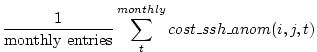
- Map out
- Map out
 averaged over 1 month, i.e. averaged over 1 month, i.e.
- sum over daily entries and plot daily average as function of time. i.e.
Next: 8.1.2 Hydrographic constraints
Up: 8.1 The ECCO state
Previous: 8.1 The ECCO state
Contents
mitgcm-support@dev.mitgcm.org
| Copyright © 2002
Massachusetts Institute of Technology |
 |
|