|
|
|
|


Next: 8.2 The external forcing
Up: 8.1 The ECCO state
Previous: 8.1.1 Sea surface height
Contents
Subsections
Observation of temperature and salinity from various sources are
used to constrain the model. These are:
- CTD obs. for
 , ,  from various WOCE sections from various WOCE sections
- XBT obs. for
- Sea surface temperature (SST) and salinity (SSS) from
Reynolds et al. (???)
- , from ARGO floats
- , from fields from Levitus (???)
| |
|
|
|
| field |
file name |
deccription |
unit |
| |
|
|
|
| |
|
|
|
| tbar |
tbarfile |
monthly model mean pot. temperature |
[ C] C] |
| sbar |
sbarfile |
monthly model mean salinity |
[ppt] |
| tdat |
tdatfile |
monthly mean Levitus pot. temperature |
[C] |
| sdat |
sdatfile |
monthly mean Levitus salinity |
[ppt] |
| ctdtobs |
ctdtfile |
monthly WOCE CTD pot. temperature |
[C] |
| ctdsobs |
ctdsfile |
monthly WOCE CTD salinity |
[ppt] |
| xbtobs |
xbtfile |
monthly XBT in-situ(!) temperature |
[C] |
| sstdat |
sstdatfile |
monthly Reynolds pot. SST |
[C] |
| sssdat |
sssdatfile |
monthly Reynolds SSS |
[ppt] |
| argotobs |
argotfile |
monthly ARGO in-situ(!) temperature |
[C] |
| argosobs |
argosfile |
monthly ARGO salinity |
[ppt] |
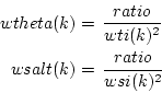
| wti, wsi |
data_errfile |
vert. stdev. profile for , |
|
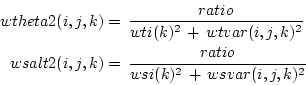
| wtvar |
temperrfile |
spatially varying stdev. |
[C] |
| wsvar |
salterrfile |
spatially varying stdev. |
[ppt] |
| |
|
|
|
![\begin{displaymath}\begin{split}cost\_xbt\_t(i,j,k) & = \, \left[ \, \frac{fac \...
...theta[xbtobs(\tau)] \right\}^2 \, \right](i,j,k) \\ \end{split}\end{displaymath}](img1966.png) |
(8.7) |
 \\ \end{split}\end{displaymath}](img1967.png) |
(8.8) |
 \\ \end{split}\end{displaymath}](img1968.png) |
(8.9) |
 \\ \end{split}\end{displaymath}](img1969.png) |
(8.10) |
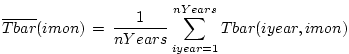
Model vs. data misfits are taken from  monthly model means
vs. Levitus monthly data.
The description below is for potential temperature.
Procedure for salinity is fully analogous.
Spatial indices monthly model means
vs. Levitus monthly data.
The description below is for potential temperature.
Procedure for salinity is fully analogous.
Spatial indices  are omitted throughout. are omitted throughout.
- Compute monthly model means for each month
 : :
- Compute misfit:
- Map out
 , ,
 . .
Next: 8.2 The external forcing
Up: 8.1 The ECCO state
Previous: 8.1.1 Sea surface height
Contents
mitgcm-support@dev.mitgcm.org
| Copyright © 2002
Massachusetts Institute of Technology |
 |
|


![$\displaystyle cost\_theta(i,j,k) \, = \, \left[
\frac{fac \cdot ratio}{wti^2} ...
...2}
\left\{ \overline{Tbar}(imon) \, - \, Tdat(imon) \right\}^2 \right] (i,j,k)
$](img1973.png)