 |
 |
|||||||||||
 |
|
|||||||||||
 |
 |
|||||||||||


|
Next: 2.9.1 Crank-Nickelson barotropic time Up: 2. Discretization and Algorithm Previous: 2.8 Non-hydrostatic formulation Contents
|
![[*]](crossref.png)
| (2.74) |
where
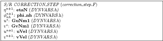
Finally, the horizontal velocities at the new time level are found by:
| (2.75) |
and the vertical velocity is found by integrating the continuity equation vertically. Note that, for the convenience of the restart procedure, the vertical integration of the continuity equation has been moved to the beginning of the time step (instead of at the end), without any consequence on the solution.
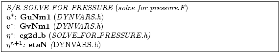
Regarding the implementation of the surface pressure solver, all
computation are done within the routine SOLVE_FOR_PRESSURE and
its dependent calls. The standard method to solve the 2D elliptic
problem (2.74) uses the conjugate gradient method (routine
CG2D); the solver matrix and conjugate gradient operator are
only function of the discretized domain and are therefore evaluated
separately, before the time iteration loop, within INI_CG2D.
The computation of the RHS ![]() is partly done in CALC_DIV_GHAT and in SOLVE_FOR_PRESSURE.
is partly done in CALC_DIV_GHAT and in SOLVE_FOR_PRESSURE.
The same method is applied for the non hydrostatic part, using a conjugate gradient 3D solver (CG3D) that is initialized in INI_CG3D. The RHS terms of 2D and 3D problems are computed together at the same point in the code.
Subsections
- 2.9.1 Crank-Nickelson barotropic time stepping
- 2.9.2 Non-linear free-surface
- 2.9.2.1 pressure/geo-potential and free surface
- 2.9.2.2 Free surface effect on column total thickness (Non-linear free-surface)
- 2.9.2.3 Tracer conservation with non-linear free-surface
- 2.9.2.4 Time stepping implementation of the non-linear free-surface
- 2.9.2.5 Non-linear free-surface and vertical resolution
Next: 2.9.1 Crank-Nickelson barotropic time Up: 2. Discretization and Algorithm Previous: 2.8 Non-hydrostatic formulation Contents mitgcm-support@dev.mitgcm.org
| Copyright © 2002 Massachusetts Institute of Technology |


