|
|
|
|


Next: 3.15 Surface Driven Convection
Up: 3.14 Held-Suarez Atmosphere MITgcm
Previous: 3.14.3 Set-up description
Contents
Subsections
3.14.4 Experiment Configuration
The model configuration for this experiment resides under the
directory verification/tutorial_held_suarez_cs. The experiment files
- input/data
- input/data.pkg
- input/eedata,
- input/data.shap,
- code/packages.conf,
- code/CPP_OPTIONS.h,
- code/SIZE.h,
- code/DIAGNOSTICS_SIZE.h,
- code/external_forcing.F,
contain the code customizations and parameter settings for these
experiments. Below we describe the customizations
to these files associated with this experiment.
This file, reproduced completely below, specifies the main parameters
for the experiment.
The parameters that are significant for this configuration are:
- Lines 7,
tRef=295.2, 295.5, 295.9, 296.3, 296.7, 297.1, 297.6, 298.1, 298.7, 299.3,

set reference values for potential temperature (in Kelvin units)
at each model level.
The entries are ordered like model level, from surface up to the top.
Density is calculated from anomalies at each level evaluated
with respect to the reference values set here.

- Line 10,
no_slip_sides=.FALSE.,
this line selects a free-slip lateral boundary condition for
the horizontal Laplacian friction operator
e.g.
 =0 along boundaries in
  and
and
 =0 along boundaries in
  .
.
- Lines 11,
no_slip_bottom=.FALSE.,
this line selects a free-slip boundary condition at the top,
in the vertical Laplacian friction operator
e.g.

- Line 12,
buoyancyRelation='ATMOSPHERIC',
this line sets the type of fluid and the type of vertical coordinate to use,
which, in this case, is air with a pressure like coordinate ( or
or  ).
).
- Line 13,
eosType='IDEALG',
Selects the Ideal gas equation of state.
- Line 15,
implicitFreeSurface=.TRUE.,
Selects the way the barotropic equation is solved, using here the implicit
free-surface formulation.

- Line 16,
exactConserv=.TRUE.,
Explicitly calculate again the surface pressure changes from
the divergence of the vertically integrated horizontal flow,
after the implicit free surface solver and filters are applied.

- Line 17
and Line 18,
 nonlinFreeSurf=4,
 select_rStar=2,
Select the Non-Linear free surface formulation, using  vertical coordinate
(here
).
Note that, except for the default (
vertical coordinate
(here
).
Note that, except for the default ( ), other values of those 2 parameters
are only permitted for testing/debuging purpose.
), other values of those 2 parameters
are only permitted for testing/debuging purpose.

- Line 21
uniformLin_PhiSurf=.FALSE.,
Select the linear relation between surface geopotential anomaly
and surface pressure anomaly to be evaluated from
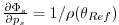 (see section 2.10.2.1).
Note that using the default (=TRUE), the constant
(see section 2.10.2.1).
Note that using the default (=TRUE), the constant  is
used instead, and is not necessary consistent with other
parts of the geopotential that relies on
is
used instead, and is not necessary consistent with other
parts of the geopotential that relies on
 .
.

- Line 23 and Line 24
 saltStepping=.FALSE.,
 momViscosity=.FALSE.,
Do not step forward Water vapour and do not compute viscous terms.
This allow to save some computer time.
- Line 25
vectorInvariantMomentum=.TRUE.,
Select the vector-invariant form to solve the momentum equation.

- Line 26
staggerTimeStep=.TRUE.,
Select the staggered time-stepping (rather than syncronous time stepping).
- Line 27 and 28
 readBinaryPrec=64,
 writeBinaryPrec=64,
Sets format for reading binary input datasets and writing output fields to
use 64-bit representation for floating-point numbers.

- Line 33,
cg2dMaxIters=200,
Sets maximum number of iterations the two-dimensional, conjugate
gradient solver will use, irrespective of convergence
criteria being met.

- Line 35,
cg2dTargetResWunit=1.E-17,
Sets the tolerance (in units of  ) which the two-dimensional,
conjugate gradient solver will use to test for convergence in equation
2.20 to
) which the two-dimensional,
conjugate gradient solver will use to test for convergence in equation
2.20 to
 .
Solver will iterate until tolerance falls below this value or until the
maximum number of solver iterations is reached.
.
Solver will iterate until tolerance falls below this value or until the
maximum number of solver iterations is reached.
- Line 40,
deltaT=450.,
Sets the timestep  used in the model to
 (
(
 ).
).

- Line 42,
startTime=124416000.,
Sets the starting time, in seconds, for the model time counter.
A non-zero starting time requires to read the initial state
from a pickup file. By default the pickup file is named according
to the integer number (nIter0) of time steps
in the startTime value (
 ).
).
- Line 44,
#nTimeSteps=69120,
A commented out setting for the length of the simulation
(in number of time-step) that corresponds to 1 year simulation.
- Line 54 and 55,
 nTimeSteps=16,
 monitorFreq=1.,
Sets the length of the simulation (in number of time-step)
and the frequency (in seconds) for "monitor" output.
to 16 iterations and 1 seconds respectively. This choice
corresponds to a short simulation test.
- Line 48,
pChkptFreq=31104000.,
Sets the time interval, in seconds, bewteen 2 consecutive
"permanent" pickups ("permanent checkpoint frequency")
that are used to restart the simuilation, to 1 year.
- Line 49,
chkptFreq=2592000.,
Sets the time interval, in seconds, bewteen 2 consecutive
"temporary" pickups ("checkpoint frequency") to 1 month.
The "temporary" pickup file name is alternatively "ckptA"
and "ckptB" ; thoses pickup (as opposed to the permanent ones)
are designed to be over-written by the model as the simulation
progresses.
- Line 50,
dumpFreq=2592000.,
Set the frequencies (in seconds) for the snap-shot output
to 1 month.
- Line 51,
#monitorFreq=43200.,
A commented out line setting the frequency (in seconds) for the
"monitor" output to 12.h. This frequency fits
better the longer simulation of 1 year.
- Line 60,
usingCurvilinearGrid=.TRUE.,
Set the horizontal type of grid to Curvilinear-Grid.
- Line 61,
horizGridFile='grid_cs32',
Set the root for the grid file name to "grid_cs32".
The grid-file names are derived from the root, adding a
suffix with the face number (e.g.: .face001.bin,
.face002.bin
)

- Lines 63 and XXX,
 delR=20*50.E2,
 Ro_SeaLevel=1.E5,
Those 2 lines define the vertical discretization, in pressure units.
The  one sets the increments in pressure units (Pa),
to 20 equally thick levels of
one sets the increments in pressure units (Pa),
to 20 equally thick levels of
 each.
The
each.
The  one sets the reference pressure at the sea-level,
to
one sets the reference pressure at the sea-level,
to
 . This define the origin (interface
  )
of the vertical pressure axis, with decreasing pressure
as the level index
)
of the vertical pressure axis, with decreasing pressure
as the level index  increases.

- Line 68,
#topoFile='topo.cs.bin'
This commented out line would allow to set the file name
of a 2-D orography file, in meters units, to 'topo.cs.bin'.

other lines in the file input/data are standard values
that are described in the MITgcm Getting Started and MITgcm Parameters
notes.
     1	# ====================
     2	# | Model parameters |
     3	# ====================
     4	#
     5	# Continuous equation parameters
     6	 &PARM01
     7	 tRef=295.2, 295.5, 295.9, 296.3, 296.7, 297.1, 297.6, 298.1, 298.7, 299.3,
     8	      300.0, 300.7, 301.9, 304.1, 308.0, 315.1, 329.5, 362.3, 419.2, 573.8,
     9	 sRef=20*0.0,
    10	 no_slip_sides=.FALSE.,
    11	 no_slip_bottom=.FALSE.,
    12	 buoyancyRelation='ATMOSPHERIC',
    13	 eosType='IDEALG',
    14	 rotationPeriod=86400.,
    15	 implicitFreeSurface=.TRUE.,
    16	 exactConserv=.TRUE.,
    17	 nonlinFreeSurf=4,
    18	 select_rStar=2,
    19	 hFacInf=0.2,
    20	 hFacSup=2.0,
    21	 uniformLin_PhiSurf=.FALSE.,
    22	#hFacMin=0.2,
    23	 saltStepping=.FALSE.,
    24	 momViscosity=.FALSE.,
    25	 vectorInvariantMomentum=.TRUE.,
    26	 staggerTimeStep=.TRUE.,
    27	 readBinaryPrec=64,
    28	 writeBinaryPrec=64,
    29	 &
    30
    31	# Elliptic solver parameters
    32	 &PARM02
    33	 cg2dMaxIters=200,
    34	#cg2dTargetResidual=1.E-12,
    35	 cg2dTargetResWunit=1.E-17,
    36	 &
    37
    38	# Time stepping parameters
    39	 &PARM03
    40	 deltaT=450.,
    41	#nIter0=276480,
    42	 startTime=124416000.,
    43	#- run for 1 year (192.iterations x 450.s = 1.day, 360*192=69120):
    44	#nTimeSteps=69120,
    45	#forcing_In_AB=.FALSE.,
    46	 tracForcingOutAB=1,
    47	 abEps=0.1,
    48	 pChkptFreq=31104000.,
    49	 chkptFreq=2592000.,
    50	 dumpFreq=2592000.,
    51	#monitorFreq=43200.,
    52	 taveFreq=0.,
    53	#- to run a short test (2.h):
    54	 nTimeSteps=16,
    55	 monitorFreq=1.,
    56	 &
    57
    58	# Gridding parameters
    59	 &PARM04
    60	 usingCurvilinearGrid=.TRUE.,
    61	 horizGridFile='grid_cs32',
    62	 radius_fromHorizGrid=6370.E3,
    63	 delR=20*50.E2,
    64	 &
    65
    66	# Input datasets
    67	 &PARM05
    68	#topoFile='topo.cs.bin',
    69	 &
This file, reproduced completely below, specifies the additional
packages that the model uses for the experiment. Note that some
packages are used by default (e.g.: pkg/generic_advdiff) and
some others are selected according to parameter in input/data
(e.g.: pkg/mom_vecinv).
The additional packages that are used for this configuration are
- Line 3,
useSHAP_FILT=.TRUE.,
This line selects the Shapiro filter Shapiro [1970]
(pkg/shap_filt) to be used in this experiment.
- Line 4,
useDiagnostics=.TRUE.,
This line selects the pkg/diagnostics
to be used in this experiment.
- Line 5,
#useMNC=.TRUE.,
This line that would selects the pkg/mnc for I/O
is commented out.
The entire file input/data.pkg is reproduced here below:
     1	# Packages
     2	 &PACKAGES
     3	 useSHAP_FILT=.TRUE.,
     4	 useDiagnostics=.TRUE.,
     5	#useMNC=.TRUE.,
     6	 &
This file uses standard default values except line 6:
useCubedSphereExchange=.TRUE.,
This line selects the cubed-sphere specific exchanges to
to connect tiles and faces edges.
This file, reproduced completely below, specifies the parameters
that the model uses for the Shapiro filter package (Shapiro [1970],
section 2.20).
The parameters that are significant for this configuration are:
The entire file input/data.shap is reproduced here below:
     1	# Shapiro Filter parameters
     2	 &SHAP_PARM01
     3	 shap_filt_uvStar=.FALSE.,
     4	 shap_filt_TrStagg=.TRUE.,
     5	 Shap_funct=2,
     6	 nShapT=0,
     7	 nShapUV=4,
     8	#nShapTrPhys=0,
     9	 nShapUVPhys=4,
    10	#Shap_TrLength=140000.,
    11	#Shap_uvLength=110000.,
    12	#Shap_Trtau=5400.,
    13	#Shap_uvtau=1800.,
    14	#Shap_diagFreq=2592000.,
    15	 &
Four lines are customized in this file for the current experiment
- Line 39,
sNx=32,
sets the lateral domain extent in grid points along the x-direction,
for 1 face.
- Line 40,
sNy=32,
sets the lateral domain extent in grid points along the y-direction,
for 1 face.
- Line 43,
nSx=6,
sets the number of tiles in the x-direction, for the model domain
decomposition. In this simple case (one processor and 1 tile per
face), this number corresponds to the total number of faces.
- Line 49,
Nr=20,
sets the vertical domain extent in grid points.
This file, reproduced completely below, specifies the packages
that are compiled and made available for this experiment.
The additional packages that are used for this configuration are
- Line 4,
gfd
This line selects the standard set of packages that are used by default.
- Line 5,
shap_filt
This line makes the Shapiro filter package available for this
experiment.
- Line 6,
exch2
This line selects the exch2 pacakge to be compiled and
used in this experiment. Note that, with the present structure of
the model, the parameter useEXCH2 does not exists and
therefore, this package is always used when it is compiled.
- Line 7,
diagnostics
This line selects the pkg/diagnostics to be compiled,
and makes it available for this experiment.
- Line 8,
mnc
This line selects the pkg/mnc to be compiled,
and makes it available for this experiment.
The entire file code/packages.conf is reproduced here below:
     1	# $Header: /u/gcmpack/MITgcm/verification/tutorial_held_suarez_cs/code/packages.conf,v 1.2 2014/08/20 20:24:09 jmc Exp $
     2	# $Name:  $
     3
     4	gfd
     5	shap_filt
     6	exch2
     7	diagnostics
     8	mnc
This file uses standard default except for Line 40
(diff CPP_OPTIONS.h ../../../model/inc):
#define NONLIN_FRSURF
This line allow to use the non-linear free-surface part of the code,
which is required for the
coordinate formulation.
Other files relevant to this experiment are
- code/external_forcing.F
- input/grid_cs32.face00[n].bin, with
contain the code customisations and binary input files for this
experiments. Below we describe the customisations
to these files associated with this experiment.
The file code/external_forcing.F contains 4 subroutines
that calculate the forcing terms (Right-Hand side term) in the
momentum equation (3.61,
S/R EXTERNAL_FORCING_U and EXTERNAL_FORCING_V)
and in the potential temperature equation
(3.62, S/R EXTERNAL_FORCING_T).
The water-vapour forcing subroutine (S/R EXTERNAL_FORCING_S)
is left empty for this experiment.
The grid-files input/grid_cs32.face00[n].bin, with
,
are binary files (direct-access, big-endian 64.bits real) that
contains all the cubed-sphere grid lengths, areas and grid-point
positions, with one file per face.
Each file contains 18 2-D arrays (dimension
 ) that correspond
to the model variables:
XC YC DXF DYF RA XG YG DXV DYU RAZ DXC DYC RAW RAS DXG DYG AngleCS AngleSN
(see GRID.h file)
) that correspond
to the model variables:
XC YC DXF DYF RA XG YG DXV DYU RAZ DXC DYC RAW RAS DXG DYG AngleCS AngleSN
(see GRID.h file)
Next: 3.15 Surface Driven Convection
Up: 3.14 Held-Suarez Atmosphere MITgcm
Previous: 3.14.3 Set-up description
Contents
mitgcm-support@mitgcm.org
| Copyright © 2006
Massachusetts Institute of Technology |
Last update 2018-01-23 |
 |
|


