


Next: 3.14.4 Experiment Configuration
Up: 3.14 Held-Suarez Atmosphere MITgcm
Previous: 3.14.2 Forcing
Contents
Subsections
The model is configured in hydrostatic form, using non-boussinesq
 coordinate.
The vertical resolution is uniform,
coordinate.
The vertical resolution is uniform,
 ,
with 20 levels, from
,
with 20 levels, from
 to 0
at the top.
The domain is discretised using C32 cube-sphere grid [Adcroft et al., 2004a]
that cover the whole sphere with a relatively uniform grid-spacing.
The resolution at the equator or along the Greenwitch meridian
is similar to the
to 0
at the top.
The domain is discretised using C32 cube-sphere grid [Adcroft et al., 2004a]
that cover the whole sphere with a relatively uniform grid-spacing.
The resolution at the equator or along the Greenwitch meridian
is similar to the
 equaly spaced longitude-latitude grid,
but requires
equaly spaced longitude-latitude grid,
but requires  less grid points.
Grid spacing and grid-point location are not computed by the model but
read from files.
less grid points.
Grid spacing and grid-point location are not computed by the model but
read from files.
The vector-invariant form of the momentum equation (see section
2.15) is used so that no explicit
metrics are necessary.
Applying the vector-invariant discretization to the
atmospheric equations 1.59, and adding the
forcing term
(3.61, 3.62)
on the right-hand-side,
leads to the set of equations that are solved in this configuration:
 KE KE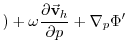 |
 |
 |
(3.65) |
 |
|
0 |
(3.66) |
 |
|
0 |
(3.67) |
 |
|
![$\displaystyle -k_{\theta}[\theta-\theta_{eq}]$](img1511.png) |
(3.68) |
where
 and
and
 are the horizontal velocity vector and the vertical velocity in pressure coordinate,
 is the relative vorticity and
  the Coriolis parameter,
 is the vertical unity vector,
KE is the kinetic energy,
is the vertical unity vector,
KE is the kinetic energy,  is the geopotential
and
is the geopotential
and  the Exner function
(
the Exner function
(
 ).
Variables marked with ' corresponds to anomaly from
the resting, uniformly stratified state.
).
Variables marked with ' corresponds to anomaly from
the resting, uniformly stratified state.
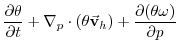
As described in MITgcm Numerical Solution Procedure 2,
the continuity equation is integrated vertically, to give a prognostic
equation for the surface pressure  :
:
 |
(3.69) |
The implicit free surface form of the pressure equation described in
Marshall et al. [1997b] is employed to solve for
;
Integrating vertically the hydrostatic balance
gives the geopotential  and allow to step forward the momentum equation
3.65.
The potential temperature,
and allow to step forward the momentum equation
3.65.
The potential temperature,  , is stepped forward using the
new velocity field (staggered time-step, section
2.8).
, is stepped forward using the
new velocity field (staggered time-step, section
2.8).
The numerical stability for inertial oscillations
Adcroft [1995]
 |
|
|
(3.70) |
evaluates to
 at the poles,
for
at the poles,
for
 ,
which is well below the
,
which is well below the  upper limit for stability.
The advective CFL Adcroft [1995]
for a extreme maximum horizontal flow speed of
 and the smallest horizontal grid spacing
 :
:
 |
|
|
(3.71) |
evaluates to  , which is close to the stability
limit of 0.5.
, which is close to the stability
limit of 0.5.
The stability parameter for internal gravity waves propagating
with a maximum speed of
 Adcroft [1995]
 |
|
|
(3.72) |
evaluates to
 . This is close to the linear
stability limit of 0.5.
. This is close to the linear
stability limit of 0.5.
Next: 3.14.4 Experiment Configuration
Up: 3.14 Held-Suarez Atmosphere MITgcm
Previous: 3.14.2 Forcing
Contents
mitgcm-support@mitgcm.org
| Copyright © 2006
Massachusetts Institute of Technology |
Last update 2018-01-23 |
 |
|


