 |
 |
|||||||||||
 |
|
|||||||||||
 |
 |
|||||||||||


|
Next: 4.3.2 Starting the code Up: 4.3 Using the WRAPPER Previous: 4.3 Using the WRAPPER Contents Subsections
|
|
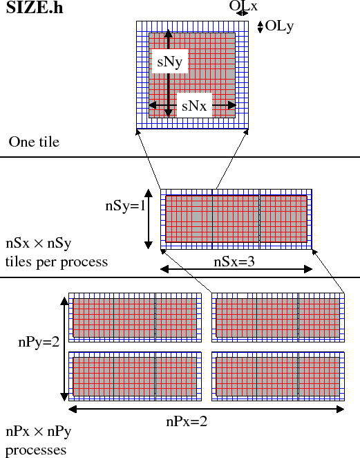
The parameters nSx and nSy specify the number of tiles that will be created within a single process. Each of these tiles will have internal dimensions of sNx and sNy. If, when the code is executed, these tiles are allocated to different threads of a process that are then bound to different physical processors ( see the multi-threaded execution discussion in section 4.3.2 ) then computation will be performed concurrently on each tile. However, it is also possible to run the same decomposition within a process running a single thread on a single processor. In this case the tiles will be computed over sequentially. If the decomposition is run in a single process running multiple threads but attached to a single physical processor, then, in general, the computation for different tiles will be interleaved by system level software. This too is a valid mode of operation.
The parameters sNx, sNy, OLx, OLy, nSx andnSy are used extensively by numerical code. The settings of sNx, sNy, OLx and OLy are used to form the loop ranges for many numerical calculations and to provide dimensions for arrays holding numerical state. The nSx andnSy are used in conjunction with the thread number parameter myThid. Much of the numerical code operating within the WRAPPER takes the form
      DO bj=myByLo(myThid),myByHi(myThid)
       DO bi=myBxLo(myThid),myBxHi(myThid)
          :
          a block of computations ranging
          over 1,sNx +/- OLx and 1,sNy +/- OLy grid points
          :
       ENDDO
      ENDDO

      communication code to sum a number or maybe update
      tile overlap regions

      DO bj=myByLo(myThid),myByHi(myThid)
       DO bi=myBxLo(myThid),myBxHi(myThid)
          :
          another block of computations ranging
          over 1,sNx +/- OLx and 1,sNy +/- OLy grid points
          :
       ENDDO
      ENDDO
The variables myBxLo(myThid), myBxHi(myThid), myByLo(myThid) and myByHi(myThid) set the bounds of the loops in bi and bj in this
schematic. These variables specify the subset of the tiles in
the range 1,nSx and 1,nSy that the logical processor bound to
thread number myThid owns. The thread number variable myThid
ranges from 1 to the total number of threads requested at execution time.
For each value of myThid the loop scheme above will step sequentially
through the tiles owned by that thread. However, different threads will
have different ranges of tiles assigned to them, so that separate threads can
compute iterations of the bi, bj loop concurrently.
Within a bi, bj loop
computation is performed concurrently over as many processes and threads
as there are physical processors available to compute.
An exception to the the use of bi and bj in loops arises in the exchange routines used when the exch2 package is used with the cubed sphere. In this case bj is generally set to 1 and the loop runs from 1,bi. Within the loop bi is used to retrieve the tile number, which is then used to reference exchange parameters.
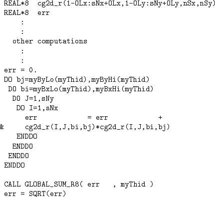
The amount of computation that can be embedded a single loop over bi and bj varies for different parts of the MITgcm algorithm. Figure 4.10 shows a code extract from the two-dimensional implicit elliptic solver. This portion of the code computes the l2Norm of a vector whose elements are held in the array cg2d_r writing the final result to scalar variable err. In this case, because the l2norm requires a global reduction, the bi,bj loop only contains one statement. This computation phase is then followed by a communication phase in which all threads and processes must participate. However, in other areas of the MITgcm code entries subsections of code are within a single bi,bj loop. For example the evaluation of all the momentum equation prognostic terms ( see S/R DYNAMICS()) is within a single bi,bj loop.
 |
The final decomposition parameters are nPx and nPy. These parameters
are used to indicate to the WRAPPER level how many processes (each with
nSx![]() nSy tiles) will be used for this simulation.
This information is needed during initialization and during I/O phases.
However, unlike the variables sNx, sNy, OLx, OLy, nSx and nSy
the values of nPx and nPy are absent
from the core numerical and support code.
nSy tiles) will be used for this simulation.
This information is needed during initialization and during I/O phases.
However, unlike the variables sNx, sNy, OLx, OLy, nSx and nSy
the values of nPx and nPy are absent
from the core numerical and support code.
4.3.1.1 Examples of SIZE.h specifications
The following different SIZE.h parameter setting illustrate how to interpret the values of sNx, sNy, OLx, OLy, nSx, nSy, nPx and nPy.
      PARAMETER (
     &           sNx =  90,
     &           sNy =  40,
     &           OLx =   3,
     &           OLy =   3,
     &           nSx =   1,
     &           nSy =   1,
     &           nPx =   1,
     &           nPy =   1)
This sets up a single tile with x-dimension of ninety grid points, y-dimension of forty grid points, and x and y overlaps of three grid points each.PARAMETER ( & sNx = 45, & sNy = 20, & OLx = 3, & OLy = 3, & nSx = 1, & nSy = 1, & nPx = 2, & nPy = 2)This sets up tiles with x-dimension of forty-five grid points, y-dimension of twenty grid points, and x and y overlaps of three grid points each. There are four tiles allocated to four separate processes (nPx=2,nPy=2) and arranged so that the global domain size is again ninety grid points in x and forty grid points in y. In general the formula for global grid size (held in model variables Nx and Ny) isNx = sNx*nSx*nPx Ny = sNy*nSy*nPyPARAMETER ( & sNx = 90, & sNy = 10, & OLx = 3, & OLy = 3, & nSx = 1, & nSy = 2, & nPx = 1, & nPy = 2)This sets up tiles with x-dimension of ninety grid points, y-dimension of ten grid points, and x and y overlaps of three grid points each. There are four tiles allocated to two separate processes (nPy=2) each of which has two separate sub-domains nSy=2, The global domain size is again ninety grid points in x and forty grid points in y. The two sub-domains in each process will be computed sequentially if they are given to a single thread within a single process. Alternatively if the code is invoked with multiple threads per process the two domains in y may be computed concurrently.PARAMETER ( & sNx = 32, & sNy = 32, & OLx = 3, & OLy = 3, & nSx = 6, & nSy = 1, & nPx = 1, & nPy = 1)This sets up tiles with x-dimension of thirty-two grid points, y-dimension of thirty-two grid points, and x and y overlaps of three grid points each. There are six tiles allocated to six separate logical processors (nSx=6). This set of values can be used for a cube sphere calculation. Each tile of size represents a face of the
cube. Initializing the tile connectivity correctly ( see section
4.3.3.3. allows the rotations associated with
moving between the six cube faces to be embedded within the
tile-tile communication code.
represents a face of the
cube. Initializing the tile connectivity correctly ( see section
4.3.3.3. allows the rotations associated with
moving between the six cube faces to be embedded within the
tile-tile communication code.
Next: 4.3.2 Starting the code Up: 4.3 Using the WRAPPER Previous: 4.3 Using the WRAPPER Contents mitgcm-support@mitgcm.org
| Copyright © 2006 Massachusetts Institute of Technology | Last update 2018-01-23 |


