 |
 |
|||||||||||
 |
|
|||||||||||
 |
 |
|||||||||||


|
Next: 6.4.2 KPP: Nonlocal K-Profile Up: 6.4 Ocean Packages Previous: 6.4 Ocean Packages Contents Subsections
|
| (6.1) |
where
 |
(6.2) |
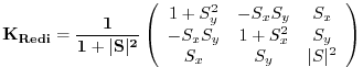
Here,
The first point to note is that a typical slope in the ocean interior
is small, say of the order ![]() . A maximum slope might be of
order
. A maximum slope might be of
order ![]() and only exceeds such in unstratified regions where
the slope is ill defined. It is therefore justifiable, and
customary, to make the small slope approximation,
and only exceeds such in unstratified regions where
the slope is ill defined. It is therefore justifiable, and
customary, to make the small slope approximation, ![]() . The Redi
projection tensor then becomes:
. The Redi
projection tensor then becomes:
 |
(6.3) |
6.4.1.2 GM parameterization
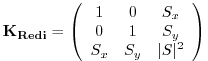
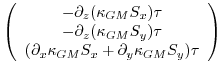
The GM parameterization aims to represent the ``advective'' or
``transport'' effect of geostrophic eddies by means of a ``bolus''
velocity,
![]() . The divergence of this advective flux is added
to the tracer tendency equation (on the rhs):
. The divergence of this advective flux is added
to the tracer tendency equation (on the rhs):
| (6.4) |
The bolus velocity
![]() is defined as the rotational of a
streamfunction
is defined as the rotational of a
streamfunction
![]() =
=
![]() :
:
 |
(6.5) |
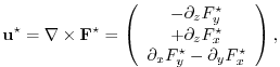
and thus is automatically non-divergent. In the GM parameterization, the streamfunction is specified in terms of the isoneutral slopes
| (6.6) | |||
| (6.7) |
with boundary conditions
 |
(6.8) |
This is the form of the GM parameterization as applied by Donabasaglu, 1997, in MOM versions 1 and 2.
Note that in the MITgcm, the variables containing the GM bolus streamfunction are:
| (6.9) |
6.4.1.3 Griffies Skew Flux
Griffies [1998] notes that the discretisation of bolus velocities involves
multiple layers of differencing and interpolation that potentially
lead to noisy fields and computational modes. He pointed out that the
bolus flux can be re-written in terms of a non-divergent flux and a
skew-flux:
 |
|||
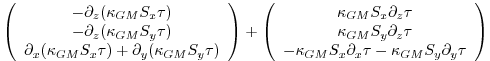 |
The first vector is non-divergent and thus has no effect on the tracer field and can be dropped. The remaining flux can be written:
| (6.10) |
where
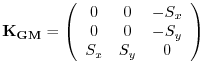 |
(6.11) |
is an anti-symmetric tensor.
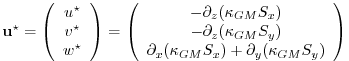
This formulation of the GM parameterization involves fewer derivatives than the original and also involves only terms that already appear in the Redi mixing scheme. Indeed, a somewhat fortunate cancellation becomes apparent when we use the GM parameterization in conjunction with the Redi isoneutral mixing scheme:
| (6.12) |
In the instance that
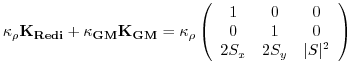 |
(6.13) |
which differs from the variable Laplacian diffusion tensor by only two non-zero elements in the
6.4.1.4 Variable

Visbeck et al. [1997] suggest making the eddy coefficient,
![]() , a function of the Eady growth rate,
, a function of the Eady growth rate,
![]() . The formula involves a non-dimensional constant,
. The formula involves a non-dimensional constant,
![]() , and a length-scale
, and a length-scale ![]() :
:
where the Eady growth rate has been depth averaged (indicated by the over-line). A local Richardson number is defined
where
6.4.1.5 Tapering and stability
Experience with the GFDL model showed that the GM scheme has to be matched to the convective parameterization. This was originally expressed in connection with the introduction of the KPP boundary layer scheme [Large et al., 1994] but in fact, as subsequent experience with the MIT model has found, is necessary for any convective parameterization.
|
Slope clipping
Deep convection sites and the mixed layer are indicated by
homogenized, unstable or nearly unstable stratification. The slopes in
such regions can be either infinite, very large with a sign reversal
or simply very large. From a numerical point of view, large slopes
lead to large variations in the tensor elements (implying large bolus
flow) and can be numerically unstable. This was first recognized by
Cox [1987] who implemented ``slope clipping'' in the isopycnal mixing
tensor. Here, the slope magnitude is simply restricted by an upper
limit:
| (6.14) | |||
| (6.15) | |||
| (6.16) | |||
| (6.17) |
Notice that this algorithm assumes stable stratification through the ``min'' function. In the case where the fluid is well stratified (
| (6.18) |
while in the limited regions (
| (6.19) |
so that the slope magnitude is limited
The slope clipping scheme is activated in the model by setting GM_taper_scheme = 'clipping' in data.gmredi.
Even using slope clipping, it is normally the case that the vertical
diffusion term (with coefficient
![]() ) is large and must be time-stepped using an
implicit procedure (see section on discretisation and code later).
Fig. 6.8 shows the mixed layer depth resulting from
a) using the GM scheme with clipping and b) no GM scheme (horizontal
diffusion). The classic result of dramatically reduced mixed layers is
evident. Indeed, the deep convection sites to just one or two points
each and are much shallower than we might prefer. This, it turns out,
is due to the over zealous re-stratification due to the bolus transport
parameterization. Limiting the slopes also breaks the adiabatic nature
of the GM/Redi parameterization, re-introducing diabatic fluxes in
regions where the limiting is in effect.
) is large and must be time-stepped using an
implicit procedure (see section on discretisation and code later).
Fig. 6.8 shows the mixed layer depth resulting from
a) using the GM scheme with clipping and b) no GM scheme (horizontal
diffusion). The classic result of dramatically reduced mixed layers is
evident. Indeed, the deep convection sites to just one or two points
each and are much shallower than we might prefer. This, it turns out,
is due to the over zealous re-stratification due to the bolus transport
parameterization. Limiting the slopes also breaks the adiabatic nature
of the GM/Redi parameterization, re-introducing diabatic fluxes in
regions where the limiting is in effect.
Tapering: Gerdes, Koberle and Willebrand, Clim. Dyn. 1991
The tapering scheme used in Gerdes et al. [1991] addressed two issues with the clipping method: the introduction of large vertical fluxes in addition to convective adjustment fluxes is avoided by tapering the GM/Redi slopes back to zero in low-stratification regions; the adjustment of slopes is replaced by a tapering of the entire GM/Redi tensor. This means the direction of fluxes is unaffected as the amplitude is scaled.
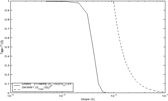
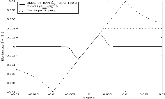
The scheme inserts a tapering function, ![]() , in front of the
GM/Redi tensor:
, in front of the
GM/Redi tensor:
![$\displaystyle f_1(S) = \min \left[ 1, \left( \frac{S_{max}}{\vert S\vert}\right)^2 \right]$](img2100.png) |
(6.20) |
where
The GKW91 tapering scheme is activated in the model by setting GM_taper_scheme = 'gkw91' in data.gmredi.
Tapering: Danabasoglu and McWilliams, J. Clim. 1995
The tapering scheme used by Danabasoglu and McWilliams [1995] followed a similar procedure but used a different
tapering function, ![]() :
:
| (6.21) |
where
The DM95 tapering scheme is activated in the model by setting GM_taper_scheme = 'dm95' in data.gmredi.
Tapering: Large, Danabasoglu and Doney, JPO 1997
The tapering used in Large et al. [1997] is based on the
DM95 tapering scheme, but also tapers the scheme with an additional
function of height, ![]() , so that the GM/Redi SGS fluxes are
reduced near the surface:
, so that the GM/Redi SGS fluxes are
reduced near the surface:
| (6.22) |
where
The LDD97 tapering scheme is activated in the model by setting GM_taper_scheme = 'ldd97' in data.gmredi.
6.4.1.6 Package Reference
------------------------------------------------------------------------
<-Name->|Levs|<-parsing code->|<--  Units   -->|<- Tile (max=80c)
------------------------------------------------------------------------
GM_VisbK|  1 |SM P    M1      |m^2/s           |Mixing coefficient from Visbeck etal parameterization
GM_Kux  | 15 |UU P 177MR      |m^2/s           |K_11 element (U.point, X.dir) of GM-Redi tensor
GM_Kvy  | 15 |VV P 176MR      |m^2/s           |K_22 element (V.point, Y.dir) of GM-Redi tensor
GM_Kuz  | 15 |UU   179MR      |m^2/s           |K_13 element (U.point, Z.dir) of GM-Redi tensor
GM_Kvz  | 15 |VV   178MR      |m^2/s           |K_23 element (V.point, Z.dir) of GM-Redi tensor
GM_Kwx  | 15 |UM   181LR      |m^2/s           |K_31 element (W.point, X.dir) of GM-Redi tensor
GM_Kwy  | 15 |VM   180LR      |m^2/s           |K_32 element (W.point, Y.dir) of GM-Redi tensor
GM_Kwz  | 15 |WM P    LR      |m^2/s           |K_33 element (W.point, Z.dir) of GM-Redi tensor
GM_PsiX | 15 |UU   184LR      |m^2/s           |GM Bolus transport stream-function : X component
GM_PsiY | 15 |VV   183LR      |m^2/s           |GM Bolus transport stream-function : Y component
GM_KuzTz| 15 |UU   186MR      |degC.m^3/s      |Redi Off-diagonal Tempetature flux: X component
GM_KvzTz| 15 |VV   185MR      |degC.m^3/s      |Redi Off-diagonal Tempetature flux: Y component
6.4.1.7 Experiments and tutorials that use gmredi
- Global Ocean tutorial, in tutorial_global_oce_latlon verification directory, described in section 3.12
- Front Relax experiment, in front_relax verification directory.
- Ideal 2D Ocean experiment, in ideal_2D_oce verification directory.
Next: 6.4.2 KPP: Nonlocal K-Profile Up: 6.4 Ocean Packages Previous: 6.4 Ocean Packages Contents mitgcm-support@mitgcm.org
| Copyright © 2006 Massachusetts Institute of Technology | Last update 2018-01-23 |


