Home Contact Us Site Map  
 
       
    next up previous contents
Next: 6.4.3 GGL90: a TKE Up: 6.4 Ocean Packages Previous: 6.4.1 GMREDI: Gent-McWilliams/Redi SGS   Contents

Subsections

6.4.2 KPP: Nonlocal K-Profile Parameterization for Vertical Mixing

Authors: Dimitris Menemenlis and Patrick Heimbach


6.4.2.1 Introduction

The nonlocal K-Profile Parameterization (KPP) scheme of Large et al. [1994] unifies the treatment of a variety of unresolved processes involved in vertical mixing. To consider it as one mixing scheme is, in the view of the authors, somewhat misleading since it consists of several entities to deal with distinct mixing processes in the ocean's surface boundary layer, and the interior:

  1. mixing in the interior is goverened by shear instability (modeled as function of the local gradient Richardson number), internal wave activity (assumed constant), and double-diffusion (not implemented here).
  2. a boundary layer depth $ h$ or hbl is determined at each grid point, based on a critical value of turbulent processes parameterized by a bulk Richardson number;
  3. mixing is strongly enhanced in the boundary layer under the stabilizing or destabilizing influence of surface forcing (buoyancy and momentum) enabling boundary layer properties to penetrate well into the thermocline; mixing is represented through a polynomial profile whose coefficients are determined subject to several contraints;
  4. the boundary-layer profile is made to agree with similarity theory of turbulence and is matched, in the asymptotic sense (function and derivative agree at the boundary), to the interior thus fixing the polynomial coefficients; matching allows for some fraction of the boundary layer mixing to affect the interior, and vice versa;
  5. a ``non-local'' term $ \hat{\gamma}$ or ghat which is independent of the vertical property gradient further enhances mixing where the water column is unstable
The scheme has been extensively compared to observations (see e.g. Large et al. [1997]) and is now coomon in many ocean models.

The current code originates in the NCAR NCOM 1-D code and was kindly provided by Bill Large and Jan Morzel. It has been adapted first to the MITgcm vector code and subsequently to the current parallel code. Adjustment were mainly in conjunction with WRAPPER requirements (domain decomposition and threading capability), to enable automatic differentiation of tangent linear and adjoint code via TAMC.

The following sections will describe the KPP package configuration and compiling (6.4.2.2), the settings and choices of runtime parameters (6.4.2.3), more detailed description of equations to which these parameters relate (6.4.2.4), and key subroutines where they are used (6.4.2.5), and diagnostics output of KPP-derived diffusivities, viscosities and boundary-layer/mixed-layer depths (6.4.2.6).


6.4.2.2 KPP configuration and compiling

As with all MITgcm packages, KPP can be turned on or off at compile time

  • using the packages.conf file by adding kpp to it,
  • or using genmake2 adding -enable=kpp or -disable=kpp switches
  • Required packages and CPP options:
    No additional packages are required, but the MITgcm kernel flag enabling the penetration of shortwave radiation below the surface layer needs to be set in CPP_OPTIONS.h as follows:
    #define SHORTWAVE_HEATING
(see Section 3.4).

Parts of the KPP code can be enabled or disabled at compile time via CPP preprocessor flags. These options are set in KPP_OPTIONS.h. Table 6.4.2.2 summarizes them.


Table 6.6:  
CPP option Description
_KPP_RL  
FRUGAL_KPP  
KPP_SMOOTH_SHSQ  
KPP_SMOOTH_DVSQ  
KPP_SMOOTH_DENS  
KPP_SMOOTH_VISC  
KPP_SMOOTH_DIFF  
KPP_ESTIMATE_UREF  
INCLUDE_DIAGNOSTICS_INTERFACE_CODE  
KPP_GHAT  
EXCLUDE_KPP_SHEAR_MIX  


6.4.2.3 Run-time parameters

Run-time parameters are set in files data.pkg and data.kpp which are read in kpp_readparms.F. Run-time parameters may be broken into 3 categories: (i) switching on/off the package at runtime, (ii) required MITgcm flags, (iii) package flags and parameters.

6.4.2.3.1 Enabling the package

 
The KPP package is switched on at runtime by setting useKPP = .TRUE. in data.pkg.

6.4.2.3.2 Required MITgcm flags

 
The following flags/parameters of the MITgcm dynamical kernel need to be set in conjunction with KPP:

implicitViscosity = .TRUE. enable implicit vertical viscosity
implicitDiffusion = .TRUE. enable implicit vertical diffusion

6.4.2.3.3 Package flags and parameters

 
Table 6.4.2.3 summarizes the runtime flags that are set in data.pkg, and their default values.


Table 6.7:  
Flag/parameter default Description
I/O related parameters
kpp_freq deltaTClock Recomputation frequency for KPP fields
kpp_dumpFreq dumpFreq Dump frequency of KPP field snapshots
kpp_taveFreq taveFreq Averaging and dump frequency of KPP fields
KPPmixingMaps .FALSE. include KPP diagnostic maps in STDOUT
KPPwriteState .FALSE. write KPP state to file
KPP_ghatUseTotalDiffus .FALSE. if .T. compute non-local term using total vertical diffusivity
    if .F. use KPP vertical diffusivity
Genral KPP parameters
minKPPhbl delRc(1) Minimum boundary layer depth
epsilon 0.1 nondimensional extent of the surface layer
vonk 0.4 von Karman constant
dB_dz 5.2E-5 1/s$ ^2$ maximum dB/dz in mixed layer hMix
concs 98.96  
concv 1.8  
Boundary layer parameters (S/R bldepth)
Ricr 0.3 critical bulk Richardson number
cekman 0.7 coefficient for Ekman depth
cmonob 1.0 coefficient for Monin-Obukhov depth
concv 1.8 ratio of interior to entrainment depth buoyancy frequency
hbf 1.0 fraction of depth to which absorbed solar radiation contributes
    to surface buoyancy forcing
Vtc   non-dim. coeff. for velocity scale of turbulant velocity shear
    ( = function of concv,concs,epsilon,vonk,Ricr)
Boundary layer mixing parameters (S/R blmix)
cstar 10. proportionality coefficient for nonlocal transport
cg   non-dimensional coefficient for counter-gradient term
    ( = function of cstar,vonk,concs,epsilon)
Interior mixing parameters (S/R Ri_iwmix)
Riinfty 0.7 gradient Richardson number limit for shear instability
BVDQcon -0.2E-4 1/s$ ^2$ Brunt-Väisalä squared
difm0 0.005 m$ ^2$ /s viscosity max. due to shear instability
difs0 0.005 m$ ^2$ /s tracer diffusivity max. due to shear instability
dift0 0.005 m$ ^2$ /s heat diffusivity max. due to shear instability
difmcon 0.1 viscosity due to convective instability
difscon 0.1 tracer diffusivity due to convective instability
diftcon 0.1 heat diffusivity due to convective instability
Double-diffusive mixing parameters (S/R ddmix)
Rrho0 not used limit for double diffusive density ratio
dsfmax not used maximum diffusivity in case of salt fingering


6.4.2.4 Equations and key routines

We restrict ourselves to writing out only the essential equations that relate to main processes and parameters mentioned above. We closely follow the notation of Large et al. [1994].

6.4.2.4.1 KPP_CALC:

Top-level routine.
 

6.4.2.4.2 KPP_MIX:

Intermediate-level routine
 

6.4.2.4.3 BLMIX: Mixing in the boundary layer
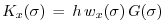


The vertical fluxes $ \overline{wx}$ of momentum and tracer properties $ X$ is composed of a gradient-flux term (proportional to the vertical property divergence $ \partial_z X$ ), and a ``nonlocal'' term $ \gamma_x$ that enhances the gradient-flux mixing coefficient $ K_x$

$\displaystyle \overline{wx}(d) \, = \, -K_x \left( \frac{\partial X}{\partial z} \, - \, \gamma_x \right)$ (6.23)

  • Boundary layer mixing profile
    It is expressed as the product of the boundary layer depth $ h$ , a depth-dependent turbulent velocity scale $ w_x(\sigma)$ and a non-dimensional shape function $ G(\sigma)$

    $\displaystyle K_x(\sigma) \, = \, h \, w_x(\sigma) \, G(\sigma)$ (6.24)

    with dimensionless vertical coordinate $ \sigma = d/h$ . For details of $ w_x(\sigma)$ and $ G(\sigma)$ we refer to Large et al. [1994].

  • Nonlocal mixing term
    The nonlocal transport term $ \gamma$ is nonzero only for tracers in unstable (convective) forcing conditions. Thus, depending on the stability parameter $ \zeta = d/L$ (with depth $ d$ , Monin-Obukhov length scale $ L$ ) it has the following form:
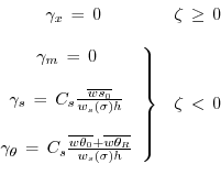
    \begin{displaymath}\begin{array}{cl}
\gamma_x \, = \, 0 & \zeta \, \ge \, 0 \\
...
...) h} \\
\end{array}\right\}
&
\zeta \, < \, 0 \\
\end{array}\end{displaymath}     (6.25)

In practice, the routine peforms the following tasks:

  1. compute velocity scales at hbl
  2. find the interior viscosities and derivatives at hbl
  3. compute turbulent velocity scales on the interfaces
  4. compute the dimensionless shape functions at the interfaces
  5. compute boundary layer diffusivities at the interfaces
  6. compute nonlocal transport term
  7. find diffusivities at kbl-1 grid level

6.4.2.4.4 RI_IWMIX: Mixing in the interior

 
Compute interior viscosity and diffusivity coefficients due to
  • shear instability (dependent on a local gradient Richardson number),
  • to background internal wave activity, and
  • to static instability (local Richardson number $ <$ 0).

TO BE CONTINUED.

6.4.2.4.5 BLDEPTH: Boundary layer depth calculation:

 
The oceanic planetary boundary layer depth, hbl, is determined as the shallowest depth where the bulk Richardson number is equal to the critical value, Ricr.

Bulk Richardson numbers are evaluated by computing velocity and buoyancy differences between values at zgrid(kl) < 0 and surface reference values. In this configuration, the reference values are equal to the values in the surface layer. When using a very fine vertical grid, these values should be computed as the vertical average of velocity and buoyancy from the surface down to epsilon*zgrid(kl).

When the bulk Richardson number at k exceeds Ricr, hbl is linearly interpolated between grid levels zgrid(k) and zgrid(k-1).

The water column and the surface forcing are diagnosed for stable/ustable forcing conditions, and where hbl is relative to grid points (caseA), so that conditional branches can be avoided in later subroutines.

TO BE CONTINUED.

6.4.2.4.6 KPP_CALC_DIFF_T/_S, KPP_CALC_VISC:

 
Add contribution to net diffusivity/viscosity from KPP diffusivity/viscosity.

TO BE CONTINUED.

6.4.2.4.7 KPP_TRANSPORT_T/_S/_PTR:

 
Add non local KPP transport term (ghat) to diffusive temperature/salinity/passive tracer flux. The nonlocal transport term is nonzero only for scalars in unstable (convective) forcing conditions.

TO BE CONTINUED.

6.4.2.4.8 Implicit time integration

 
TO BE CONTINUED.

6.4.2.4.9 Penetration of shortwave radiation

 
TO BE CONTINUED.


6.4.2.5 Flow chart

C     !CALLING SEQUENCE:
c ...
c  kpp_calc (TOP LEVEL ROUTINE)
c  |
c  |-- statekpp: o compute all EOS/density-related arrays
c  |             o uses S/R FIND_ALPHA, FIND_BETA, FIND_RHO
c  |
c  |-- kppmix
c  |   |--- ri_iwmix (compute interior mixing coefficients due to constant
c  |   |              internal wave activity, static instability, 
c  |   |              and local shear instability).
c  |   |
c  |   |--- bldepth (diagnose boundary layer depth)
c  |   |
c  |   |--- blmix (compute boundary layer diffusivities)
c  |   |
c  |   |--- enhance (enhance diffusivity at interface kbl - 1)
c  |   o
c  |
c  |-- swfrac
c  o


6.4.2.6 KPP diagnostics

Diagnostics output is available via the diagnostics package (see Section 7.1). Available output fields are summarized here:

------------------------------------------------------
 <-Name->|Levs|grid|<--  Units   -->|<- Tile (max=80c)
------------------------------------------------------
 KPPviscA| 23 |SM  |m^2/s           |KPP vertical eddy viscosity coefficient
 KPPdiffS| 23 |SM  |m^2/s           |Vertical diffusion coefficient for salt & tracers
 KPPdiffT| 23 |SM  |m^2/s           |Vertical diffusion coefficient for heat
 KPPghat | 23 |SM  |s/m^2           |Nonlocal transport coefficient
 KPPhbl  |  1 |SM  |m               |KPP boundary layer depth, bulk Ri criterion
 KPPmld  |  1 |SM  |m               |Mixed layer depth, dT=.8degC density criterion
 KPPfrac |  1 |SM  |                |Short-wave flux fraction penetrating mixing layer

6.4.2.7 Reference experiments

lab_sea:

natl_box:

6.4.2.8 References


6.4.2.9 Experiments and tutorials that use kpp

  • Labrador Sea experiment, in lab_sea verification directory


next up previous contents
Next: 6.4.3 GGL90: a TKE Up: 6.4 Ocean Packages Previous: 6.4.1 GMREDI: Gent-McWilliams/Redi SGS   Contents
mitgcm-support@mitgcm.org
Copyright © 2006 Massachusetts Institute of Technology Last update 2018-01-23