 |
 |
|||||||||||
 |
|
|||||||||||
 |
 |
|||||||||||


|
Next: 6.6.3 SHELFICE Package Up: 6.6 Sea Ice Packages Previous: 6.6.1 THSICE: The Thermodynamic Contents Subsections
|
|||||||||||||||||||||||||||||||||||||||||||||||||||||||||||||||||||||||||||||||||||||||||||||||||||||||||||||||||||||||||||||||||||||||||||||||||||||||||||||||||||||||||||||||||||||||||||||||||||||||||||||||||||||||||||||||||||||||||||||||||||||||||||||||||||||||||||||||||||||||||||||||||||||||||||||||||||||||||||||||||||||||||||||||||||||||||||||||||||||||||||||||||||||||||||||||||||||||||||||||||||||||||||||||||||||||||||||||||||||||||||||||||||||||||||||||||||||||||||||||
| Name | Default value | Description | Reference |
|---|---|---|---|
| SEAICEwriteState | T | write sea ice state to file | |
| SEAICEuseDYNAMICS | T | use dynamics | |
| SEAICEuseJFNK | F | use the JFNK-solver | |
| SEAICEuseTEM | F | use truncated ellipse method | |
| SEAICEuseStrImpCpl | F | use strength implicit coupling in LSR/JFNK | |
| SEAICEuseMetricTerms | T | use metric terms in dynamics | |
| SEAICEuseEVPpickup | T | use EVP pickups | |
| SEAICEuseFluxForm | F | use flux form for 2nd central difference advection scheme | |
| SEAICErestoreUnderIce | F | enable restoring to climatology under ice | |
| useHB87stressCoupling | F | turn on ice-ocean stress coupling following Hibler and Bryan [1987] | |
| usePW79thermodynamics | T | flag to turn off zero-layer-thermodynamics for testing | |
| SEAICEadvHeff/Area/Snow/Salt | T | flag to turn off advection of scalar state variables | |
| SEAICEuseFlooding | T | use flood-freeze algorithm | |
| SEAICE_no_slip | F | switch between free-slip and no-slip boundary conditions | |
| SEAICE_deltaTtherm | dTracerLev(1) | thermodynamic timestep | |
| SEAICE_deltaTdyn | dTracerLev(1) | dynamic timestep | |
| SEAICE_deltaTevp | 0 | EVP sub-cycling time step, values |
|
| SEAICEuseEVPstar | F | use modified EVP* instead of EVP | |
| SEAICEuseEVPrev | F | use yet another variation on EVP* | |
| SEAICEnEVPstarSteps | UNSET | number of modified EVP* iteration | |
| SEAICE_evpAlpha | UNSET | EVP* parameter | |
| SEAICE_evpBeta | UNSET | EVP* parameter | |
| SEAICEaEVPcoeff | UNSET | aEVP parameter | |
| SEAICEaEVPcStar | 4 | aEVP parameter | [Kimmritz et al., 2016] |
| SEAICEaEVPalphaMin | 5 | aEVP parameter | [Kimmritz et al., 2016] |
| SEAICE_elasticParm |
|
EVP paramter |
|
| SEAICE_evpTauRelax |
|
relaxation time scale |
|
| SEAICEnewtonIterMax | 10 | maximum number of JFNK-Newton iterations | |
| SEAICEkrylovIterMax | 10 | maximum number of JFNK-Krylov iterations | |
| SEAICE_JFNK_lsIter | (off) | start line search after ``lsIter'' Newton iterations | |
| JFNKgamma_nonlin | 1.0E-05 | non-linear tolerance parameter for JFNK solver | |
| JFNKgamma_lin_min/max | 0.10/0.99 | tolerance parameters for linear JFNK solver | |
| JFNKres_tFac | UNSET | tolerance parameter for FGMRES residual | |
| SEAICE_JFNKepsilon | 1.0E-06 | step size for the FD-Jacobian-times-vector | |
| SEAICE_dumpFreq | dumpFreq | dump frequency | |
| SEAICE_taveFreq | taveFreq | time-averaging frequency | |
| SEAICE_dump_mdsio | T | write snap-shot using MDSIO | |
| SEAICE_tave_mdsio | T | write TimeAverage using MDSIO | |
| SEAICE_dump_mnc | F | write snap-shot using MNC | |
| SEAICE_tave_mnc | F | write TimeAverage using MNC | |
| SEAICE_initialHEFF | 0.00000E+00 | initial sea-ice thickness | |
| SEAICE_drag | 2.00000E-03 | air-ice drag coefficient | |
| OCEAN_drag | 1.00000E-03 | air-ocean drag coefficient | |
| SEAICE_waterDrag | 5.50000E+00 | water-ice drag | |
| SEAICE_dryIceAlb | 7.50000E-01 | winter albedo | |
| SEAICE_wetIceAlb | 6.60000E-01 | summer albedo | |
| SEAICE_drySnowAlb | 8.40000E-01 | dry snow albedo | |
| SEAICE_wetSnowAlb | 7.00000E-01 | wet snow albedo | |
| SEAICE_waterAlbedo | 1.00000E-01 | water albedo | |
| SEAICE_strength | 2.75000E+04 | sea-ice strength |
|
| SEAICE_cStar | 20.0000E+00 | sea-ice strength paramter |
|
| SEAICE_rhoAir | 1.3 (or exf value) | density of air (kg/m |
|
| SEAICE_cpAir | 1004 (or exf value) | specific heat of air (J/kg/K) | |
| SEAICE_lhEvap | 2,500,000 (or exf value) | latent heat of evaporation | |
| SEAICE_lhFusion | 334,000 (or exf value) | latent heat of fusion | |
| SEAICE_lhSublim | 2,834,000 | latent heat of sublimation | |
| SEAICE_dalton | 1.75E-03 | sensible heat transfer coefficient | |
| SEAICE_iceConduct | 2.16560E+00 | sea-ice conductivity | |
| SEAICE_snowConduct | 3.10000E-01 | snow conductivity | |
| SEAICE_emissivity | 5.50000E-08 | Stefan-Boltzman | |
| SEAICE_snowThick | 1.50000E-01 | cutoff snow thickness | |
| SEAICE_shortwave | 3.00000E-01 | penetration shortwave radiation | |
| SEAICE_freeze | -1.96000E+00 | freezing temp. of sea water | |
| SEAICE_saltFrac | 0.0 | salinity newly formed ice (fraction of ocean surface salinity) | |
| SEAICE_frazilFrac | 0.0 | Fraction of surface level negative heat content anomalies (relative to the local freezing point) | |
| SEAICEstressFactor | 1.00000E+00 | scaling factor for ice-ocean stress | |
| Heff/Area/HsnowFile/Hsalt | UNSET | initial fields for variables HEFF/AREA/HSNOW/HSALT | |
| LSR_ERROR | 1.00000E-04 | sets accuracy of LSR solver | |
| DIFF1 | 0.0 | parameter used in advect.F | |
| HO | 5.00000E-01 | demarcation ice thickness (AKA lead closing paramter |
|
| MAX_HEFF | 1.00000E+01 | maximum ice thickness | |
| MIN_ATEMP | -5.00000E+01 | minimum air temperature | |
| MIN_LWDOWN | 6.00000E+01 | minimum downward longwave | |
| MAX_TICE | 3.00000E+01 | maximum ice temperature | |
| MIN_TICE | -5.00000E+01 | minimum ice temperature | |
| IMAX_TICE | 10 | iterations for ice heat budget | |
| SEAICE_EPS | 1.00000E-10 | reduce derivative singularities | |
| SEAICE_area_reg | 1.00000E-5 | minimum concentration to regularize ice thickness | |
| SEAICE_hice_reg | 0.05 m | minimum ice thickness for regularization | |
| SEAICE_multDim | 1 | number of ice categories for thermodynamics | |
| SEAICE_useMultDimSnow | F | use SEAICE_multDim snow categories |
6.6.2.3.3 Input fields and units
- HeffFile:
- Initial sea ice thickness averaged over grid cell in meters; initializes variable HEFF;
- AreaFile:
- Initial fractional sea ice cover, range
![$ [0,1]$](img2704.png) ;
initializes variable AREA;
;
initializes variable AREA;
- HsnowFile:
- Initial snow thickness on sea ice averaged over grid cell in meters; initializes variable HSNOW;
- HsaltFile:
- Initial salinity of sea ice averaged over grid
cell in g/m
 ; initializes variable HSALT;
6.6.2.4 Description
[TO BE CONTINUED/MODIFIED]
The MITgcm sea ice model (MITgcm/sim) is based on a variant of the viscous-plastic (VP) dynamic-thermodynamic sea ice model [Zhang and Hibler, 1997] first introduced by Hibler [1980,1979]. In order to adapt this model to the requirements of coupled ice-ocean state estimation, many important aspects of the original code have been modified and improved [Losch et al., 2010]:
- the code has been rewritten for an Arakawa C-grid, both B- and C-grid variants are available; the C-grid code allows for no-slip and free-slip lateral boundary conditions;
- three different solution methods for solving the nonlinear momentum equations have been adopted: LSOR [Zhang and Hibler, 1997], EVP [Hunke and Dukowicz, 1997], JFNK [Losch et al., 2014; Lemieux et al., 2010];
- ice-ocean stress can be formulated as in Hibler and Bryan [1987] or as in Campin et al. [2008];
- ice variables are advected by sophisticated, conservative advection schemes with flux limiting;
- growth and melt parameterizations have been refined and extended in order to allow for more stable automatic differentiation of the code.
The ice dynamics models that are most widely used for large-scale climate studies are the viscous-plastic (VP) model [Hibler, 1979], the cavitating fluid (CF) model [Flato and Hibler, 1992], and the elastic-viscous-plastic (EVP) model [Hunke and Dukowicz, 1997]. Compared to the VP model, the CF model does not allow ice shear in calculating ice motion, stress, and deformation. EVP models approximate VP by adding an elastic term to the equations for easier adaptation to parallel computers. Because of its higher accuracy in plastic solution and relatively simpler formulation, compared to the EVP model, we decided to use the VP model as the default dynamic component of our ice model. To do this we extended the line successive over relaxation (LSOR) method of Zhang and Hibler [1997] for use in a parallel configuration. An EVP model and a free-drift implemtation can be selected with runtime flags.
6.6.2.4.1 Compatibility with ice-thermodynamics package thsice
Note, that by default the seaice-package includes the orginial so-called zero-layer thermodynamics following Hibler [1980] with a snow cover as in Zhang et al. [1998]. The zero-layer thermodynamic model assumes that ice does not store heat and, therefore, tends to exaggerate the seasonal variability in ice thickness. This exaggeration can be significantly reduced by using Semtner's [1976] three-layer thermodynamic model that permits heat storage in ice. Recently, the three-layer thermodynamic model has been reformulated by Winton [2000]. The reformulation improves model physics by representing the brine content of the upper ice with a variable heat capacity. It also improves model numerics and consumes less computer time and memory.
The Winton sea-ice thermodynamics have been ported to the MIT GCM; they currently reside under pkg/thsice. The package thsice is described in section 6.6.1; it is fully compatible with the packages seaice and exf. When turned on together with seaice, the zero-layer thermodynamics are replaced by the Winton thermodynamics. In order to use the seaice-package with the thermodynamics of thsice, compile both packages and turn both package on in data.pkg; see an example in global_ocean.cs32x15/input.icedyn. Note, that once thsice is turned on, the variables and diagnostics associated to the default thermodynamics are meaningless, and the diagnostics of thsice have to be used instead.
6.6.2.4.2 Surface forcing
The sea ice model requires the following input fields: 10-m winds, 2-m air temperature and specific humidity, downward longwave and shortwave radiations, precipitation, evaporation, and river and glacier runoff. The sea ice model also requires surface temperature from the ocean model and the top level horizontal velocity. Output fields are surface wind stress, evaporation minus precipitation minus runoff, net surface heat flux, and net shortwave flux. The sea-ice model is global: in ice-free regions bulk formulae are used to estimate oceanic forcing from the atmospheric fields.
6.6.2.4.3 Dynamics
The momentum equation of the sea-ice model is
where
where
6.6.2.4.4 Viscous-Plastic (VP) Rheology
For an isotropic system the stress tensor
The ice strain rate is given by
The maximum ice pressure
with the constants
|
with the abbreviation
| ||
The bulk viscosities are bounded above by imposing both a minimum
Defining the CPP-flag SEAICE_ZETA_SMOOTHREG in
SEAICE_OPTIONS.h before compiling replaces the method for
bounding ![]() by a smooth (differentiable) expression:
by a smooth (differentiable) expression:
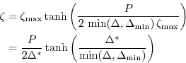
where
6.6.2.4.5 LSR and JFNK solver
In the matrix notation, the discretized momentum equations can be written as
The solution vector
In order to overcome the poor convergence of the Picard-solver,
Lemieux et al. [2010] introduced a Jacobian-free Newton-Krylov solver for
the sea ice momentum equations. This solver is also implemented in the
MITgcm [Losch et al., 2014]. The Newton method transforms minimizing
the residual
![]() to finding the roots of a multivariate Taylor
expansion of the residual
to finding the roots of a multivariate Taylor
expansion of the residual
![]() around the previous (
around the previous (![]() ) estimate
) estimate
![]() :
:
with the Jacobian
for
Forming the Jacobian
![]() explicitly is often avoided as ``too
error prone and time consuming'' [Knoll and Keyes, 2004]. Instead,
Krylov methods only require the action of
explicitly is often avoided as ``too
error prone and time consuming'' [Knoll and Keyes, 2004]. Instead,
Krylov methods only require the action of
![]() on an arbitrary
vector
on an arbitrary
vector
![]() and hence allow a matrix free algorithm for solving
Eq.(6.45) [Knoll and Keyes, 2004]. The action of
and hence allow a matrix free algorithm for solving
Eq.(6.45) [Knoll and Keyes, 2004]. The action of
![]() can be approximated by a first-order Taylor series expansion:
can be approximated by a first-order Taylor series expansion:
or computed exactly with the help of automatic differentiation (AD) tools. SEAICE_JFNKepsilon sets the step size
We use the Flexible Generalized Minimum RESidual method
[FGMRES, Saad, 1993] with right-hand side preconditioning
to solve Eq.(6.45) iteratively starting from a first
guess of
![]() . For the preconditioning matrix
. For the preconditioning matrix
![]() we choose a simplified form of the system matrix
we choose a simplified form of the system matrix
![]() [Lemieux et al., 2010] where
[Lemieux et al., 2010] where
![]() is
the estimate of the previous Newton step
is
the estimate of the previous Newton step ![]() . The transformed
equation(6.45) becomes
. The transformed
equation(6.45) becomes
The Krylov method iteratively improves the approximate solution to (6.47) in subspace (
To use the JFNK-solver set SEAICEuseJFNK = .TRUE. in the
namelist file data.seaice; SEAICE_ALLOW_JFNK needs to
be defined in SEAICE_OPTIONS.h and we recommend using a smooth
regularization of ![]() by defining SEAICE_ZETA_SMOOTHREG
(see above) for better convergence. The non-linear Newton iteration
is terminated when the
by defining SEAICE_ZETA_SMOOTHREG
(see above) for better convergence. The non-linear Newton iteration
is terminated when the ![]() -norm of the residual is reduced by
-norm of the residual is reduced by
![]() (runtime parameter JFNKgamma_nonlin =
1.e-4 will already lead to expensive simulations) with respect to
the initial norm:
(runtime parameter JFNKgamma_nonlin =
1.e-4 will already lead to expensive simulations) with respect to
the initial norm:
![]() . Within a non-linear
iteration, the linear FGMRES solver is terminated when the residual is
smaller than
. Within a non-linear
iteration, the linear FGMRES solver is terminated when the residual is
smaller than
![]() where
where ![]() is
determined by
is
determined by
so that the linear tolerance parameter
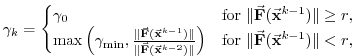
Setting SEAICEuseStrImpCpl = .TRUE., turns on ``strength implicit coupling'' [Hutchings et al., 2004] in the LSR-solver and in the LSR-preconditioner for the JFNK-solver. In this mode, the different contributions of the stress divergence terms are re-ordered in order to increase the diagonal dominance of the system matrix. Unfortunately, the convergence rate of the LSR solver is increased only slightly, while the JFNK-convergence appears to be unaffected.
6.6.2.4.6 Elastic-Viscous-Plastic (EVP) Dynamics
Hunke and Dukowicz [1997]'s introduced an elastic contribution to the strain rate in order to regularize Eq. 6.40 in such a way that the resulting elastic-viscous-plastic (EVP) and VP models are identical at steady state,
The EVP-model uses an explicit time stepping scheme with a short timestep. According to the recommendation of Hunke and Dukowicz [1997], the EVP-model should be stepped forward in time 120 times (
Here, the elastic parameter
To use the EVP solver, make sure that both SEAICE_CGRID and
SEAICE_ALLOW_EVP are defined in SEAICE_OPTIONS.h
(default). The solver is turned on by setting the sub-cycling time
step SEAICE_deltaTevp to a value larger than zero. The
choice of this time step is under debate. Hunke and Dukowicz [1997] recommend
order(120) time steps for the EVP solver within one model time step
![]() (deltaTmom). One can also choose order(120) time
steps within the forcing time scale, but then we recommend adjusting
the damping time scale
(deltaTmom). One can also choose order(120) time
steps within the forcing time scale, but then we recommend adjusting
the damping time scale ![]() accordingly, by setting either
SEAICE_elasticParm (
accordingly, by setting either
SEAICE_elasticParm (![]() ), so that
), so that
![]() forcing time scale
, or directly
SEAICE_evpTauRelax (
forcing time scale
, or directly
SEAICE_evpTauRelax (![]() ) to the forcing time scale.
) to the forcing time scale.
6.6.2.4.7 More stable variants of Elastic-Viscous-Plastic Dynamics:
EVP* , mEVP, and aEVP
The genuine EVP schemes appears to give noisy solutions [Bouillon et al., 2013; Lemieux et al., 2012; Hunke, 2001]. This has lead to a modified EVP or EVP* [Bouillon et al., 2013; Kimmritz et al., 2015; Lemieux et al., 2012]; here, we refer to these variants by modified EVP (mEVP) and adaptive EVP (aEVP) [Kimmritz et al., 2016]. The main idea is to modify the ``natural'' time-discretization of the momentum equations:
where
In order to use mEVP in the MITgcm, set SEAICEuseEVPstar =
.TRUE., in data.seaice. If SEAICEuseEVPrev =.TRUE.,
the actual form of equations (6.54) and
(6.55) is used with fewer implicit terms and the factor
of ![]() dropped in the stress equations (6.51)
and (6.52). Although this modifies the original
EVP-equations, it turns out to improve convergence [Bouillon et al., 2013].
dropped in the stress equations (6.51)
and (6.52). Although this modifies the original
EVP-equations, it turns out to improve convergence [Bouillon et al., 2013].
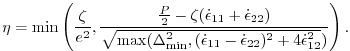
Another variant is the aEVP scheme [Kimmritz et al., 2016], where the value
of ![]() is set dynamically based on the stability criterion
is set dynamically based on the stability criterion
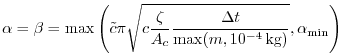
with the grid cell area
Note, that probably because of the C-grid staggering of velocities and stresses, mEVP may not converge as successfully as in Kimmritz et al. [2015], and that convergence at very high resolution (order 5km) has not been studied yet.
6.6.2.4.8 Truncated ellipse method (TEM) for yield curve
In the so-called truncated ellipse method the shear viscosity
To enable this method, set #define SEAICE_ALLOW_TEM in SEAICE_OPTIONS.h and turn it on with SEAICEuseTEM in data.seaice.
6.6.2.4.9 Ice-Ocean stress
Moving sea ice exerts a stress on the ocean which is the opposite of the stress
6.6.2.4.10 Finite-volume discretization of the stress tensor
divergence
On an Arakawa C grid, ice thickness and concentration and thus ice strength
| (6.58) | ||
| (6.59) | ||
| (6.60) | ||
so that the diagonal terms of the strain rate tensor are naturally defined at C-points and the symmetric off-diagonal term at Z-points. No-slip boundary conditions (
For a spherical polar grid, the coefficients of the metric terms are
![]() and
and
![]() , with the spherical radius
, with the spherical radius ![]() and
the latitude
and
the latitude ![]() ;
;
![]() , and
, and
![]() . For a
general orthogonal curvilinear grid,
. For a
general orthogonal curvilinear grid, ![]() and
and
![]() can be approximated by finite differences of the cell widths:
can be approximated by finite differences of the cell widths:
| (6.61) | ||
| (6.62) | ||
| (6.63) | ||
| (6.64) |
The stress tensor is given by the constitutive viscous-plastic
relation
![]() [Hibler, 1979]. The stress tensor divergence
[Hibler, 1979]. The stress tensor divergence
![]() , is
discretized in finite volumes [see
also Losch et al., 2010]. This conveniently avoids dealing with
further metric terms, as these are ``hidden'' in the differential cell
widths. For the
, is
discretized in finite volumes [see
also Losch et al., 2010]. This conveniently avoids dealing with
further metric terms, as these are ``hidden'' in the differential cell
widths. For the ![]() -equation (
-equation (![]() ) we have:
) we have:
| (6.65) | ||
with
| (6.66) | ||
| (6.67) | ||
Similarly, we have for the ![]() -equation (
-equation (![]() ):
):
| (6.68) | ||
with
| (6.69) | ||
Again, no slip boundary conditions are realized via ghost points and
![]() and
and
![]() across boundaries. For
free slip boundary conditions the lateral stress is set to zeros. In
analogy to
across boundaries. For
free slip boundary conditions the lateral stress is set to zeros. In
analogy to
![]() on boundaries, we set
on boundaries, we set
![]() , or equivalently
, or equivalently
![]() , on boundaries.
, on boundaries.
6.6.2.4.11 Thermodynamics
NOTE: THIS SECTION IS TERRIBLY OUT OF DATE
In its original formulation the sea ice model [Menemenlis et al., 2005] uses simple thermodynamics following the appendix of Semtner [1976]. This formulation does not allow storage of heat, that is, the heat capacity of ice is zero. Upward conductive heat flux is parameterized assuming a linear temperature profile and together with a constant ice conductivity. It is expressed as
The conductive heat flux depends strongly on the ice thickness ![]() .
However, the ice thickness in the model represents a mean over a
potentially very heterogeneous thickness distribution. In order to
parameterize a sub-grid scale distribution for heat flux computations,
the mean ice thickness
.
However, the ice thickness in the model represents a mean over a
potentially very heterogeneous thickness distribution. In order to
parameterize a sub-grid scale distribution for heat flux computations,
the mean ice thickness ![]() is split into
is split into ![]() thickness categories
thickness categories
![]() that are equally distributed between
that are equally distributed between ![]() and a minimum
imposed ice thickness of
and a minimum
imposed ice thickness of
![]() cm
by
cm
by
![]() for
for ![]() . The heat fluxes computed for each thickness category
is area-averaged to give the total heat flux [Hibler, 1984]. To use
this thickness category parameterization set SEAICE_multDim to
the number of desired categories (7 is a good guess, for anything
larger than 7 modify SEAICE_SIZE.h) in
data.seaice; note that this requires different restart files
and switching this flag on in the middle of an integration is not
advised. In order to include the same distribution for snow, set
SEAICE_useMultDimSnow = .TRUE.; only then, the
parameterization of always having a fraction of thin ice is efficient
and generally thicker ice is produced [Castro-Morales et al., 2014].
. The heat fluxes computed for each thickness category
is area-averaged to give the total heat flux [Hibler, 1984]. To use
this thickness category parameterization set SEAICE_multDim to
the number of desired categories (7 is a good guess, for anything
larger than 7 modify SEAICE_SIZE.h) in
data.seaice; note that this requires different restart files
and switching this flag on in the middle of an integration is not
advised. In order to include the same distribution for snow, set
SEAICE_useMultDimSnow = .TRUE.; only then, the
parameterization of always having a fraction of thin ice is efficient
and generally thicker ice is produced [Castro-Morales et al., 2014].
The atmospheric heat flux is balanced by an oceanic heat flux from
below. The oceanic flux is proportional to
![]() where
where ![]() and
and ![]() are
the density and heat capacity of sea water and
are
the density and heat capacity of sea water and ![]() is the local
freezing point temperature that is a function of salinity. This flux
is not assumed to instantaneously melt or create ice, but a time scale
of three days (run-time parameter SEAICE_gamma_t) is used
to relax
is the local
freezing point temperature that is a function of salinity. This flux
is not assumed to instantaneously melt or create ice, but a time scale
of three days (run-time parameter SEAICE_gamma_t) is used
to relax ![]() to the freezing point.
The parameterization of lateral and vertical growth of sea ice follows
that of Hibler [1980,1979]; the so-called lead closing parameter
to the freezing point.
The parameterization of lateral and vertical growth of sea ice follows
that of Hibler [1980,1979]; the so-called lead closing parameter
![]() (run-time parameter HO) has a default value of
0.5 meters.
(run-time parameter HO) has a default value of
0.5 meters.
On top of the ice there is a layer of snow that modifies the heat flux and the albedo [Zhang et al., 1998]. Snow modifies the effective conductivity according to
where
6.6.2.4.12 Advection of thermodynamic variables
Effective ice thickness (ice volume per unit area,
where
The MITgcm sea ice model provides the option to use
the thermodynamics model of Winton [2000], which in turn is based on
the 3-layer model of Semtner [1976] and which treats brine content by
means of enthalpy conservation; the corresponding package
thsice is described in section 6.6.1. This
scheme requires additional state variables, namely the enthalpy of the
two ice layers (instead of effective ice salinity), to be advected by
ice velocities.
The internal sea ice temperature is inferred from ice enthalpy. To
avoid unphysical (negative) values for ice thickness and
concentration, a positive 2nd-order advection scheme with a SuperBee
flux limiter [Roe, 1985] should be used to advect all
sea-ice-related quantities of the Winton [2000] thermodynamic model
(runtime flag thSIceAdvScheme=77 and
thSIce_diffK=![]() =0 in data.ice, defaults are 0). Because of the
non-linearity of the advection scheme, care must be taken in advecting
these quantities: when simply using ice velocity to advect enthalpy,
the total energy (i.e., the volume integral of enthalpy) is not
conserved. Alternatively, one can advect the energy content (i.e.,
product of ice-volume and enthalpy) but then false enthalpy extrema
can occur, which then leads to unrealistic ice temperature. In the
currently implemented solution, the sea-ice mass flux is used to
advect the enthalpy in order to ensure conservation of enthalpy and to
prevent false enthalpy extrema.
=0 in data.ice, defaults are 0). Because of the
non-linearity of the advection scheme, care must be taken in advecting
these quantities: when simply using ice velocity to advect enthalpy,
the total energy (i.e., the volume integral of enthalpy) is not
conserved. Alternatively, one can advect the energy content (i.e.,
product of ice-volume and enthalpy) but then false enthalpy extrema
can occur, which then leads to unrealistic ice temperature. In the
currently implemented solution, the sea-ice mass flux is used to
advect the enthalpy in order to ensure conservation of enthalpy and to
prevent false enthalpy extrema.
6.6.2.5 Key subroutines
Top-level routine: seaice_model.F
C     !CALLING SEQUENCE:
c ...
c  seaice_model (TOP LEVEL ROUTINE)
c  |
c  |-- #ifdef SEAICE_CGRID
c  |     SEAICE_DYNSOLVER
c  |     |
c  |     |-- < compute proxy for geostrophic velocity >
c  |     |
c  |     |-- < set up mass per unit area and Coriolis terms >
c  |     |
c  |     |-- < dynamic masking of areas with no ice >
c  |     |
c  |     |

c  |   #ELSE
c  |     DYNSOLVER
c  |   #ENDIF
c  |
c  |-- if ( useOBCS )
c  |     OBCS_APPLY_UVICE
c  |
c  |-- if ( SEAICEadvHeff .OR. SEAICEadvArea .OR. SEAICEadvSnow .OR. SEAICEadvSalt )
c  |     SEAICE_ADVDIFF
c  |
c  |-- if ( usePW79thermodynamics )
c  |     SEAICE_GROWTH
c  |
c  |-- if ( useOBCS )
c  |     if ( SEAICEadvHeff ) OBCS_APPLY_HEFF
c  |     if ( SEAICEadvArea ) OBCS_APPLY_AREA
c  |     if ( SEAICEadvSALT ) OBCS_APPLY_HSALT
c  |     if ( SEAICEadvSNOW ) OBCS_APPLY_HSNOW
c  |
c  |-- < do various exchanges >
c  |
c  |-- < do additional diagnostics >
c  |
c  o
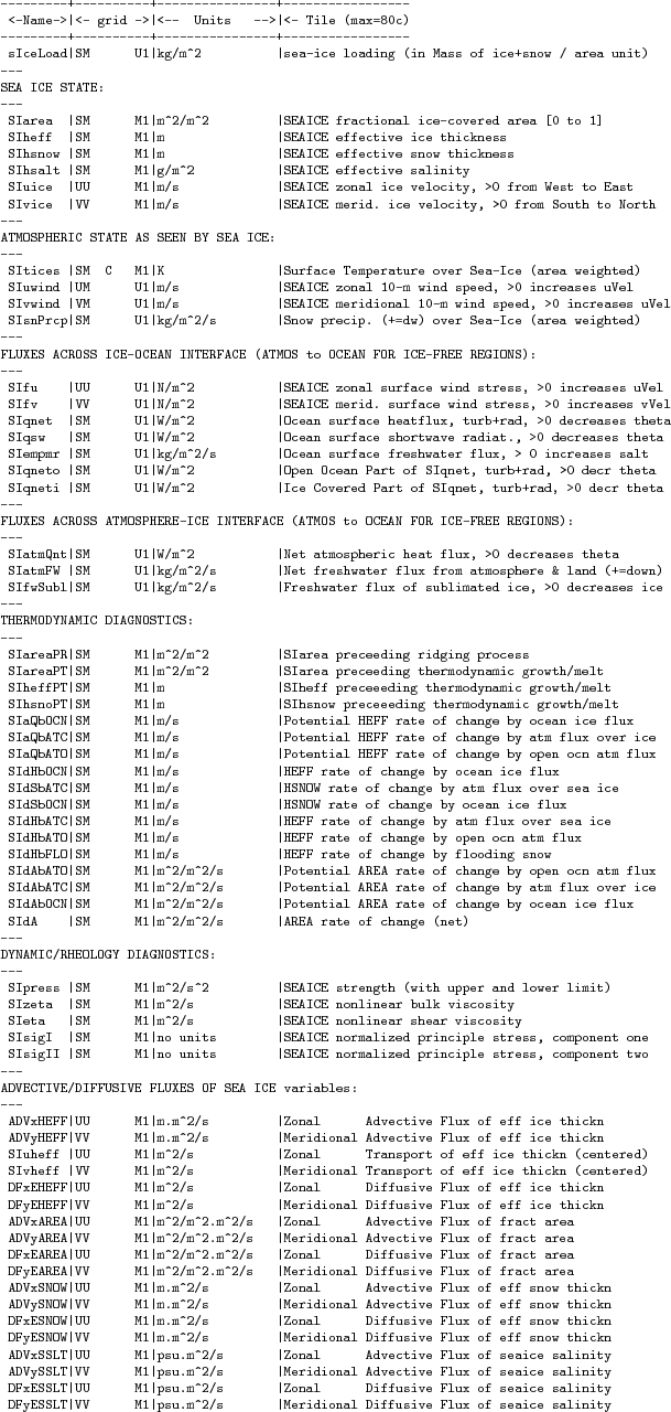
6.6.2.6 SEAICE diagnostics
Diagnostics output is available via the diagnostics package (see Section 7.1). Available output fields are summarized in Table 6.6.2.6.
6.6.2.7 Experiments and tutorials that use seaice
- Labrador Sea experiment in lab_sea verification directory.
- seaice_obcs, based on lab_sea
- offline_exf_seaice/input.seaicetd, based on lab_sea
- global_ocean.cs32x15/input.icedyn and global_ocean.cs32x15/input.seaice, global cubed-sphere-experiment with combinations of seaice and thsice
Next: 6.6.3 SHELFICE Package Up: 6.6 Sea Ice Packages Previous: 6.6.1 THSICE: The Thermodynamic Contents mitgcm-support@mitgcm.org
| Copyright © 2006 Massachusetts Institute of Technology | Last update 2018-01-23 |


