 |
 |
|||||||||||
 |
|
|||||||||||
 |
 |
|||||||||||


|
Next: 6.6.4 STREAMICE Package Up: 6.6 Sea Ice Packages Previous: 6.6.2 SEAICE Package Contents Subsections
|
|||||||||||||||||||||||||||||||||||||||||||||||||||||||||||||||||||||||||||||||||||||||||||||||||||||||||||||||
| Name | Default value | Description | Reference |
|---|---|---|---|
| useISOMIPTD | F | use simplified ISOMIP thermodynamics instead of default | |
| SHELFICEconserve | F | use conservative form of temperature boundary conditions | |
| SHELFICEboundaryLayer | F | use simple boundary layer mixing parameterization | |
| SHELFICEloadAnomalyFile | UNSET | inital geopotential anomaly | |
| SHELFICEtopoFile | UNSET | under-ice topography of ice shelves | |
| SHELFICElatentHeat | 334.0E+03 | latent heat of fusion ( |
|
| SHELFICEHeatCapacity_Cp | 2000.0E+00 | specific heat capacity of ice ( |
|
| rhoShelfIce | 917.0E+00 | (constant) mean density of ice shelf ( |
|
| SHELFICEheatTransCoeff | 1.0E-04 | transfer coefficient (exchange velocity) for temperature
( |
|
| SHELFICEsaltTransCoeff | 5.05E-03 |
transfer coefficient (exchange velocity) for salinity
( |
|
| SHELFICEkappa | 1.54E-06 | temperature diffusion coefficient of the ice shelf ( |
|
| SHELFICEthetaSurface | -20.0E+00 | (constant) surface temperature above the ice shelf ( |
|
| no_slip_shelfice | no_slip_bottom (data) | flag for slip along bottom of ice shelf | |
| SHELFICEDragLinear | bottomDragLinear (data) | linear drag coefficient at bottom ice shelf | |
| SHELFICEDragQuadratic | bottomDragQuadratic (data) | quadratic drag coefficient at bottom ice shelf | |
| SHELFICEwriteState | F | write ice shelf state to file | |
| SHELFICE_dumpFreq | dumpFreq (data) | dump frequency | |
| SHELFICE_taveFreq | taveFreq (data) | time-averaging frequency | |
| SHELFICE_tave_mnc | timeave_mnc (data.mnc) | write snap-shot using MNC | |
| SHELFICE_dump_mnc | snapshot_mnc (data.mnc) | write TimeAverage using MNC |
6.6.3.3.3 Input fields and units
- SHEFLICEtopoFile:
- under-ice topography of ice shelves in meters; upwards is positive, that as for the bathymetry files, negative values are required for topography below the sea-level;
- SHEFLICEloadAnomalyFile:
- pressure load anomaly at the bottom of
the ice shelves in pressure units (Pa); this field is absolutely
required to avoid large excursions of the free surface during
initial adjustment processes; obtained by integrating an approximate
density from the surface at
 down to the bottom of the last
fully dry cell within the ice shelf, see
Eq. (6.75); however, the file
SHEFLICEloadAnomalyFile must not be
down to the bottom of the last
fully dry cell within the ice shelf, see
Eq. (6.75); however, the file
SHEFLICEloadAnomalyFile must not be  , but
, but
 , with
 rhoConst, so that in the absenses of a
  that is different from
  , the anomaly is zero.
6.6.3.4 Description
In the light of isomorphic equations for pressure and height coordinates, the ice shelf topography on top of the water column has a similar role as (and in the language of Marshall et al. [2004] is isomorphic to) the orography and the pressure boundary conditions at the bottom of the fluid for atmospheric and oceanic models in pressure coordinates.
The total pressure ![]() in the ocean can be divided into the
pressure at the top of the water column
in the ocean can be divided into the
pressure at the top of the water column ![]() , the hydrostatic
pressure and the non-hydrostatic pressure contribution
, the hydrostatic
pressure and the non-hydrostatic pressure contribution ![]() :
:
with the gravitational acceleration
Underneath the ice shelf, the ``sea-surface height''
In the MITgcm, the total pressure anomaly ![]() which is used for
pressure gradient computations is defined by substracting a purely
depth dependent contribution
which is used for
pressure gradient computations is defined by substracting a purely
depth dependent contribution
![]() with a constant reference
density
with a constant reference
density ![]() from
from ![]() . Eq. (6.71) becomes
. Eq. (6.71) becomes
| (6.73) | |||
|
and after rearranging
| |||
| (6.74) | |||
with
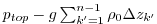
In practice, the ice shelf contribution to ![]() is computed by
integrating Eq. (6.72) from
is computed by
integrating Eq. (6.72) from ![]() to the bottom of the last
fully dry cell within the ice shelf:
to the bottom of the last
fully dry cell within the ice shelf:
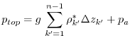
where
where
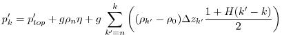
Setting SHELFICEboundaryLayer=.true. introduces a simple
boundary layer that reduces the potential noise problem at the cost of
increased vertical mixing. For this purpose the water temperature at
the ![]() -th layer abutting ice shelf topography for use in the heat
flux parameterizations is computed as a mean temperature
-th layer abutting ice shelf topography for use in the heat
flux parameterizations is computed as a mean temperature
![]() over a boundary layer of the same thickness as
the layer thickness
over a boundary layer of the same thickness as
the layer thickness
![]() :
:
where
for layers
Eq. (6.80) describes averaging over the part of the grid cell
6.6.3.4.1 Three-Equations-Thermodynamics
Freezing and melting form a boundary layer between ice shelf and
ocean. Phase transitions at the boundary between saline water and ice imply
the following fluxes across the boundary: the freshwater mass flux
![]() (
(![]() for melting); the heat flux that consists of the diffusive
flux through the ice, the latent heat flux due to melting and freezing
and the heat that is carried by the mass flux; and the salinity that
is carried by the mass flux, if the ice has a non-zero salinity
for melting); the heat flux that consists of the diffusive
flux through the ice, the latent heat flux due to melting and freezing
and the heat that is carried by the mass flux; and the salinity that
is carried by the mass flux, if the ice has a non-zero salinity ![]() .
Further, the position of the interface between ice and ocean changes
because of
.
Further, the position of the interface between ice and ocean changes
because of ![]() , so that, say, in the case of melting the volume of sea
water increases. As a consequence salinity and temperature are
modified.
, so that, say, in the case of melting the volume of sea
water increases. As a consequence salinity and temperature are
modified.
The turbulent exchange terms for tracers at the ice-ocean interface
are generally expressed as diffusive fluxes. Following
Jenkins et al. [2001], the boundary conditions for a tracer take
into account that this boundary is not a material surface.
The implied upward freshwater flux ![]() (in mass units, negative for
melting) is included in the boundary conditions for the temperature
and salinity equation as an advective flux:
(in mass units, negative for
melting) is included in the boundary conditions for the temperature
and salinity equation as an advective flux:
where tracer
In this so-called three-equation-model [e.g., Hellmer and Olbers, 1989; Jenkins et al., 2001] the heat balance at the ice-ocean interface is expressed as
where
with the salinity
where
This formulation tends to yield smaller melt rates than the simpler
formulation of the ISOMIP protocol because the freshwater flux due to
melting decreases the salinity which raises the freezing point
temperature and thus leads to less melting at the interface. For a
simpler thermodynamics model where ![]() is not computed explicitly,
for example as in the ISOMIP protocol, equation (6.81) cannot
be applied directly. In this case equation (6.84)
can be used with Eq. (6.81) to obtain:
is not computed explicitly,
for example as in the ISOMIP protocol, equation (6.81) cannot
be applied directly. In this case equation (6.84)
can be used with Eq. (6.81) to obtain:
| (6.85) |
This formulation can be used for all cases for which equation (6.84) is valid. Further, in this formulation it is obvious that melting (
The default value of SHELFICEconserve=.false. removes the
contribution
![]() from Eq. (6.81), making the
boundary conditions for temperature non-conservative.
from Eq. (6.81), making the
boundary conditions for temperature non-conservative.
6.6.3.4.2 ISOMIP-Thermodynamics
A simpler formulation follows the ISOMIP protocol (http://efdl.cims.nyu.edu/project_oisi/isomip/overview.html). The freezing and melting in the boundary layer between ice shelf and ocean is parameterized following Grosfeld et al. [1997]. In this formulation Eq. (6.82) reduces to
and the fresh water flux
In order to use this formulation, set run-time parameter useISOMIPTD=.true. in data.shelfice.
6.6.3.4.3 Remark
The shelfice package and experiments demonstrating its strenghts and weaknesses are also described in Losch [2008]. However, note that unfortunately the description of the thermodynamics in the appendix of Losch [2008] is wrong.
6.6.3.5 Key subroutines
Top-level routine: shelfice_model.F
C     !CALLING SEQUENCE:
C ...
C |-FORWARD_STEP           :: Step forward a time-step ( AT LAST !!! )
C ...
C | |-DO_OCEANIC_PHY       :: Control oceanic physics and parameterization
C ...
C | | |-SHELFICE_THERMODYNAMICS :: main routine for thermodynamics
C                                  with diagnostics
C ...
C | |-THERMODYNAMICS       :: theta, salt + tracer equations driver.
C ...
C | | |-EXTERNAL_FORCING_T :: Problem specific forcing for temperature.
C | | |-SHELFICE_FORCING_T :: apply heat fluxes from ice shelf model
C ...
C | | |-EXTERNAL_FORCING_S :: Problem specific forcing for salinity.
C | | |-SHELFICE_FORCING_S :: apply fresh water fluxes from ice shelf model
C ...
C | |-DYNAMICS             :: Momentum equations driver.
C ...
C | | |-MOM_FLUXFORM       :: Flux form mom eqn. package ( see
C ...
C | | | |-SHELFICE_U_DRAG  :: apply drag along ice shelf to u-equation
C                             with diagnostics
C ...
C | | |-MOM_VECINV         :: Vector invariant form mom eqn. package ( see
C ...
C | | | |-SHELFICE_V_DRAG  :: apply drag along ice shelf to v-equation
C                             with diagnostics
C ...
C  o
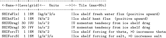
6.6.3.6 SHELFICE diagnostics
Diagnostics output is available via the diagnostics package (see Section 7.1). Available output fields are summarized in Table 6.6.3.6.
6.6.3.7 Experiments and tutorials that use shelfice
- ISOMIP, Experiment 1 (http://efdl.cims.nyu.edu/project_oisi/isomip/overview.html) in isomip verification directory.
Next: 6.6.4 STREAMICE Package Up: 6.6 Sea Ice Packages Previous: 6.6.2 SEAICE Package Contents mitgcm-support@mitgcm.org
| Copyright © 2006 Massachusetts Institute of Technology | Last update 2018-01-23 |


