|
|
|
|


Next: 2.6 Implicit time-stepping: backward
Up: 2. Discretization and Algorithm
Previous: 2.4 Pressure method with
Contents
2.5 Explicit time-stepping: Adams-Bashforth
In describing the the pressure method above we deferred describing the
time discretization of the explicit terms. We have historically used
the quasi-second order Adams-Bashforth method for all explicit terms
in both the momentum and tracer equations. This is still the default
mode of operation but it is now possible to use alternate schemes for
tracers (see section 2.17).
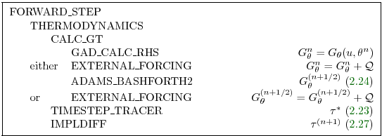
In the previous sections, we summarized an explicit scheme as:
 |
(2.23) |
where  could be any prognostic variable (
 ,
,  ,
,  or
or
 ) and
) and  is an explicit estimate of
 and would be
exact if not for implicit-in-time terms. The parenthesis about
and would be
exact if not for implicit-in-time terms. The parenthesis about  indicates that the term is explicit and extrapolated forward in time
and for this we use the quasi-second order Adams-Bashforth method:
indicates that the term is explicit and extrapolated forward in time
and for this we use the quasi-second order Adams-Bashforth method:
 |
(2.24) |
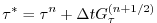
This is a linear extrapolation, forward in time, to
 . An extrapolation to the mid-point
in time,
. An extrapolation to the mid-point
in time,
 , corresponding to
 ,
would be second order accurate but is weakly unstable for oscillatory
terms. A small but finite value for
,
would be second order accurate but is weakly unstable for oscillatory
terms. A small but finite value for
 stabilizes the
method. Strictly speaking, damping terms such as diffusion and
dissipation, and fixed terms (forcing), do not need to be inside the
Adams-Bashforth extrapolation. However, in the current code, it is
simpler to include these terms and this can be justified if the flow
and forcing evolves smoothly. Problems can, and do, arise when forcing
or motions are high frequency and this corresponds to a reduced
stability compared to a simple forward time-stepping of such terms.
The model offers the possibility to leave the tracer and momentum
forcing terms and the dissipation terms outside the
Adams-Bashforth extrapolation, by turning off the logical flags
forcing_In_AB
(parameter file data, namelist PARM01, default value = True).
(tracForcingOutAB, default=0,
momForcingOutAB, default=0)
and momDissip_In_AB
(parameter file data, namelist PARM01, default value = True).
respectively.
stabilizes the
method. Strictly speaking, damping terms such as diffusion and
dissipation, and fixed terms (forcing), do not need to be inside the
Adams-Bashforth extrapolation. However, in the current code, it is
simpler to include these terms and this can be justified if the flow
and forcing evolves smoothly. Problems can, and do, arise when forcing
or motions are high frequency and this corresponds to a reduced
stability compared to a simple forward time-stepping of such terms.
The model offers the possibility to leave the tracer and momentum
forcing terms and the dissipation terms outside the
Adams-Bashforth extrapolation, by turning off the logical flags
forcing_In_AB
(parameter file data, namelist PARM01, default value = True).
(tracForcingOutAB, default=0,
momForcingOutAB, default=0)
and momDissip_In_AB
(parameter file data, namelist PARM01, default value = True).
respectively.
A stability analysis for an oscillation equation should be given at this point.
A stability analysis for a relaxation equation should be given at this point.
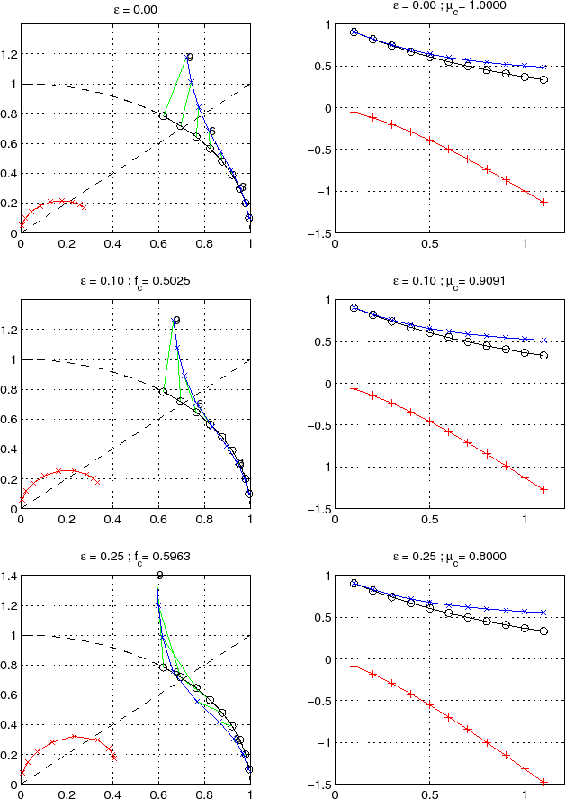
Figure 2.4:
Oscillatory and damping response of
quasi-second order Adams-Bashforth scheme for different values
of the
parameter (0., 0.1, 0.25, from top to bottom)
The analytical solution (in black), the physical mode (in blue)
and the numerical mode (in red) are represented with a CFL
step of 0.1.
The left column represents the oscillatory response
on the complex plane for CFL ranging from 0.1 up to 0.9.
The right column represents the damping response amplitude
(y-axis) function of the CFL (x-axis).
|
|
Next: 2.6 Implicit time-stepping: backward
Up: 2. Discretization and Algorithm
Previous: 2.4 Pressure method with
Contents
mitgcm-support@mitgcm.org
| Copyright © 2006
Massachusetts Institute of Technology |
Last update 2011-01-09 |
 |
|