Modeling Frozen Seas

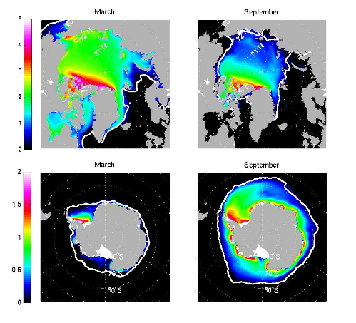
Martin Losch of the Alfred-Wegener-Institute, Bremerhaven, Germany, in collaboration with Jean Michel Campin (MIT), Patrick Heimbach (MIT), Chris Hill (MIT) and Dimitris Menemenlis (JPL) have been extending the reach of the MITgcm in to the Polar oceans, with the development of a dynamic-thermodynamic sea-ice model and its adjoint. Figure 1 shows their sea-ice thickness distribution results for the Arctic and Antarctic in opposing seasons.

Figure 1. Arctic and Antarctic results from an eddy-permitting, MITgcm, global ocean and sea-ice simulation: Sea ice thickness distribution (color, in meters) averaged over the years 1992-2002. The ice-edge (estimated as the 15% isoline of ice concentration) retrieved from passive microwave satellite data is shown as a white contour for comparison. The top row shows the results for the Arctic Ocean and the bottom row for the Antarctic Oceans; the left column shows distributions for March and the right column for September.

Based on sea-ice approaches taken in current-generation climate models, the team formulated their sea-ice model to share MITgcm’s oceanic finite-volume discretization, the Arakawa C-grid. They also incorporated many additional features and modifications that permit efficient and accurate automatic differentiation. Among these features are:

• the choice of a viscous-plastic rheology with line-successive-over-relaxation (LSOR) or an elastic-viscous-plastic (EVP) solver.
• either zero-heat-capacity or two-layer thermodynamics following Winton (2000).
• ice-ocean stress which can be optionally formulated as in Hibler and Bryan (1987).
• options for ice concentration and thickness, snow, and ice salinity or enthalpy to be advected by sophisticated conservative advection schemes with flux limiters.
• refinement and extension of growth and melt parameterizations to allow for automatic code differentiation.

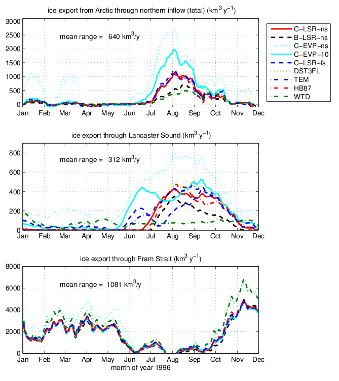
Using this sea-ice model, Losch and collaborators have carried out studies looking at the impact of model numerical formulation on simulated sea-ice characteristics. Through a series of comparison experiments they looked at differences caused by using a C-grid rather than a B-grid as well as differences resulting from solver choice (line-successive-over-relaxation (LSOR) versus elastic-viscous-plastic (EVP)). Figure 2 shows the seasonal variation in ice export volume at three different locations for the nine different experiments.

Figure 2. Inter-comparison of ice export volumes for the different experiments: Top: (through the Northern inflow), middle: (through Lancaster Sound), and bottom: (through Fram Strait). Acronyms: C-LSR-ns (baseline experiment on a C-grid, using the LSOR solver and no-slip boundary conditions), B-LSR-ns (same as baseline but with a B-grid), C-EVP-ns (same as baseline but using the EVP solver. Δt = 150s), C-EVP-10 (same as C-EVP-ns but with Δt = 10s), c-LSR-fs (same as baseline experiment but with free slip boundary conditions), DST3FL (as C-LSR-fs but using a 3rd order advection scheme and flux limiting), TEM (as C-LSR-fs but using a truncated ellipse method), HB87 (as C-LSR-fs but using Hibler and Bryan )1987) stress) and WTD (as C-LSR-fs but using Winton (2000) thermodynamics).

Figure 3 demonstrates variations in ice drift velocity. The team observed considerable sensitivity to changes in discretization (B-grid vs. C-grid) (top left panels) as well as strong sensitivity to solver technology (LSOR or EVP) (bottom left panels).

Figure 3 Ice drift velocity differences (cm/s) to the C-LSR-ns (baseline) solution averaged over the first 3-months of integration; color indicates speed differences and vectors indicate direction only. The direction vectors are smoothed and plotted for every 8th velocity point. Note the varying color scale.

Want to find out more? – contact Martin Losch.

Having worked to make their model automatically differentiable, the team were then able to capitalise on its adjoint capabilities to further probe sources of sensitivity. As an example, Figure 4 (showing snapshots of snow and ice export sensitivity with respect to ice thickness through Lancaster Sound) highlights the impact of differing boundary conditions (free-slip (left) versus no-slip (right)) on export sensitivity.

Figure 4. Snapshots of snow and ice export sensitivities through Lancaster Sound with respect to ice thickness for free-slip (left) and no-slip (right) solution (m/s)

The adjoint model provides complementary insight into causal links within the ocean/sea-ice/atmospheric forcing coupled system. The team plan to take this work further, using their model for coupled ocean/sea-ice state estimation.

Want to find out more? – contact Patrick Heimbach.

References:

Losch M., D. Menemenlis, J-M. Campin, P. Heimbach, and C. Hill. On the formulation of sea-ice models. Part 1: Effects of different solver implementations and parameterizations. Ocean Modelling, 33, 129-144, doi:10.1016/j.ocemod.2009.12.008, 2010.

Martin has been using the MITgcm since 2001. He enjoys playing the piano.

Patrick Heimbach has been working with the MITgcm since 1998. He enjoys rock-climbing and playing the cello.