 |
 |
|||||||||||
 |
|
|||||||||||
 |
 |
|||||||||||


|
Next: 6.7 Packages Related to Up: 6.6 Sea Ice Packages Previous: 6.6.3 SHELFICE Package Contents Subsections
|
| (6.91) |
where
| (6.92) |
where
| (6.93) |
is satisfied. Floatation criteria is stored in float_frac_streamice, equal to 1 where ice is at floatation.
The strain rates
![]() are generalized to the case of orthogonal
curvilinear coordinates, to include the "metric" terms that arise when casting
the equations of motion on a sphere or projection on to a sphere (see pkg/SEAICE, 6.6.2.4.8 of the MITgcm documentation). Thus
are generalized to the case of orthogonal
curvilinear coordinates, to include the "metric" terms that arise when casting
the equations of motion on a sphere or projection on to a sphere (see pkg/SEAICE, 6.6.2.4.8 of the MITgcm documentation). Thus
| (6.94) |
though the form is slightly different if a hybrid formulation is used. Whether
Again, the form is slightly different if a hybrid formulation is to be used. The scalar term multiplying
The momentum equations are solved together with appropriate boundary conditions, discussed below. In the case of a calving front boundary condition (CFBC), the boundary condition has the following form:
Here
6.6.4.2.1 Hybrid SIA-SSA stress balance
The SSA does not take vertical shear stress or strain rates (e.g.,
![]() ,
,
![]() ) into account. Although there are other
terms in the stress tensor, studies have found that in all but a few cases,
vertical shear and longitudinal stresses (represented by the SSA) are sufficient
to represent glaciological flow. streamice can allow for representation of
vertical shear, although the approximation is made that longitudinal stresses
are depth-independent. The stress balance is referred to as "hybrid" because it
is a joining of the SSA and the Shallow Ice Approximation (SIA), which only
accounts only for vertical shear. Such hybrid formulations have been shown to be
valid over a larger range of conditions than SSA (Schoof and Hindmarsh
2010, Goldberg 2011).
) into account. Although there are other
terms in the stress tensor, studies have found that in all but a few cases,
vertical shear and longitudinal stresses (represented by the SSA) are sufficient
to represent glaciological flow. streamice can allow for representation of
vertical shear, although the approximation is made that longitudinal stresses
are depth-independent. The stress balance is referred to as "hybrid" because it
is a joining of the SSA and the Shallow Ice Approximation (SIA), which only
accounts only for vertical shear. Such hybrid formulations have been shown to be
valid over a larger range of conditions than SSA (Schoof and Hindmarsh
2010, Goldberg 2011).
In the hybrid formulation,
![]() and
and
![]() , the depth-averaged
, the depth-averaged
![]() and
and ![]() velocities, replace
velocities, replace ![]() and
and ![]() in (6.88),
(6.89), and (6.90), and gradients such as
in (6.88),
(6.89), and (6.90), and gradients such as ![]() are replaced
by
are replaced
by
![]() . Viscosity becomes
. Viscosity becomes
| (6.98) |
In the formulation for
6.6.4.3 Numerical Scheme
6.6.4.3.1 Stress/momentum equations
The stress balance is solved for velocities using a very straightforward,
structured-grid finite element method. Generally a finite element method is used
to deal with irregularly shaped domains, or to deal with complicated
boundary conditions; in this case it is the latter, as explained below. (NOTE:
this is not meant as a finite element tutorial, and various mathematical objects
are defined nonrigorously. It is simply meant as an overview of the numerical
scheme used.)
In this method, the numerical velocities
![]() and
and ![]() (or
(or
![]() ,
,
![]() if a hybrid formulation) have a
bilinear shape within each cell. For instance, referring to Fig.
6.6.4.3, at a point (
if a hybrid formulation) have a
bilinear shape within each cell. For instance, referring to Fig.
6.6.4.3, at a point (![]() ) within cell (
) within cell (![]() ), and assuming a
rectangular mesh, the
), and assuming a
rectangular mesh, the ![]() velocity
velocity ![]() would be given by
would be given by
| (6.99) | ||
| (6.100) | ||
| (6.101) | ||
| (6.102) |
where
| (6.103) |
and e.g.
If we take a vector-valued function
![]() which is in the
``solution space'' of (
which is in the
``solution space'' of (![]() ) (i.e.
) (i.e. ![]() and
and ![]() are bilinear in each cell
as
defined above, and are zero where velocities are imposed), take the dot product
with by (6.88,6.89), and integrate by parts over the domain
are bilinear in each cell
as
defined above, and are zero where velocities are imposed), take the dot product
with by (6.88,6.89), and integrate by parts over the domain
![]() , we get the weak form of the momentum equation:
, we get the weak form of the momentum equation:
where
Let ![]() be the vector of all nodal values
be the vector of all nodal values
![]() that determine
that determine ![]() . If we assume that
. If we assume that ![]() and
and ![]() are independent of
are independent of ![]() ,
then for any
,
then for any
![]() , the left hand side of
(6.104) is a linear functional of
, the left hand side of
(6.104) is a linear functional of ![]() , i.e. a linear operator that
returns a scalar. We can choose
, i.e. a linear operator that
returns a scalar. We can choose ![]() and
and ![]() so that they are nonzero
only at a single node; and we can evaluate (6.104) for each such
so that they are nonzero
only at a single node; and we can evaluate (6.104) for each such
![]() and
and ![]() , giving a linearly independent set of equations for
, giving a linearly independent set of equations for
![]() and
and ![]() . The left hand side of (6.104) for each
. The left hand side of (6.104) for each ![]() and
and
![]() is
evaluated in the subroutine STREAMICE_CG_ACTION() in the source file
streamice_cg_functions.f.
The right hand side is evaluated in STREAMICE_DRIVING_STRESS(). The
latter is not a straightforward
calculation, since the thickness
is
evaluated in the subroutine STREAMICE_CG_ACTION() in the source file
streamice_cg_functions.f.
The right hand side is evaluated in STREAMICE_DRIVING_STRESS(). The
latter is not a straightforward
calculation, since the thickness ![]() and the surface
and the surface ![]() are not expressed by
piecewise bilinear functions, and is discussed below.
are not expressed by
piecewise bilinear functions, and is discussed below.
STREAMICE_CG_ACTION() represents the action of a matrix on
the vector represented by ![]() and STREAMICE_DRIVING_STRESS()
gives the right hand side of a linear system of equations. This information is
enough to solve the linear system, and this is done
with the method of conjugate gradients, implemented (with simple Jacobi
preconditioning) in STREAMICE_CG_SOLVE().
and STREAMICE_DRIVING_STRESS()
gives the right hand side of a linear system of equations. This information is
enough to solve the linear system, and this is done
with the method of conjugate gradients, implemented (with simple Jacobi
preconditioning) in STREAMICE_CG_SOLVE().
The full nonlinear system is solved in STREAMICE_VEL_SOLVE(). This
subroutine evaluates driving stress and then calls a loop
in which a sequence of linear systems is solved. After each linear solve, the
viscosity ![]() (the array visc_streamice)
and basal traction
(the array visc_streamice)
and basal traction ![]() (tau_beta_eff_streamice) is updated from
the new iterate of
(tau_beta_eff_streamice) is updated from
the new iterate of ![]() and
and ![]() . The iteration
continues until a desired tolerance is reached or the maximum number of
iterations is reached.
. The iteration
continues until a desired tolerance is reached or the maximum number of
iterations is reached.
Rather than calling STREAMICE_CG_ACTION() each iteration of the conjugate gradient, the sparse matrix can be constructed explicitly. This is done if STREAMICE_CONSTRUCT_MATRIX is #defined in STREAMICE_OPTIONS.h. This speeds up the solution because STREAMICE_CG_ACTION() contains a number of nested loops related to quadrature points and interactions between nodes of a cell.
The driving stress
![]() is not as straightforward to deal
with in the weak formulation, as
is not as straightforward to deal
with in the weak formulation, as ![]() and
and ![]() are
considered constant in a cell. Furthermore, in the ice shelf the driving stress
can be written as
are
considered constant in a cell. Furthermore, in the ice shelf the driving stress
can be written as
Among other things, this (along with equations 6.96 and 6.97) implies that for an unconfined shelf (one for which the only boundaries are a calving front and a grounding line), the stress state along the grounding line depends only on the location at depth of the grounding line. The numerical representation of velocities must respect this. Thus the driving stress contribution in the
 |
(6.106) |
where
 |
(6.107) |
6.6.4.3.2 Orthogonal curvilinear coordinates
If the grid is not rectangular, but given in orthogonal curvilinear coordinates, the evaluation of (6.104) is not exact, since the gradient of the basis functions are approximated, as we do not have complete knowledge of the coordinate system, only the grid metrics. Still, we consider nodal basis functions that are equal to 1 at a single node, and zero elsewhere in a cell.
A cell (![]() ) has separation
) has separation
![]() at the bottom and
at the bottom and
![]() at the top (referred to as dxG(i,j) and dxG(i,j+1) in the code). So, for instance, for a cell given by
at the top (referred to as dxG(i,j) and dxG(i,j+1) in the code). So, for instance, for a cell given by
![]() , the
, the ![]() -derivative of the basis function centered at (
-derivative of the basis function centered at (
![]() ) is approximated by
) is approximated by
| (6.108) |
where
Basis function derivatives and quadrature weights are stored in Dphi and grid_jacq_streamice. Both are initialized in STREAMICE_INIT_PHI, called only once.
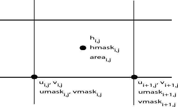
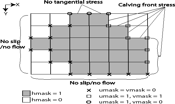
6.6.4.3.3 Boundary conditions and masks
The computational domain (which may be smaller than the array/grid as defined by SIZE.h and GRID.h) is determined by a number of mask arrays within the STREAMICE package. They are
 (STREAMICE_hmask): equal to 1 (ice-covered), 0 (open
ocean), 2 (partly-covered), or -1 (out of domain)
(STREAMICE_hmask): equal to 1 (ice-covered), 0 (open
ocean), 2 (partly-covered), or -1 (out of domain)
 (STREAMICE_umask): equal to 1 (an ``active'' velocity
node), 3 (a Dirichlet node), or 0 (zero velocity)
(STREAMICE_umask): equal to 1 (an ``active'' velocity
node), 3 (a Dirichlet node), or 0 (zero velocity)
 (STREAMICE_vmask): similar to umask
-
 (STREAMICE_ufacemaskbdry): equal to -1
(interior face), 0 (no-slip), 1 (no-stress), 2 (calving stress front), 3
(Dirichlet), or 4 (flux input boundary); when 4, then u_flux_bdry_SI must be initialized, through binary or parameter file
(STREAMICE_ufacemaskbdry): equal to -1
(interior face), 0 (no-slip), 1 (no-stress), 2 (calving stress front), 3
(Dirichlet), or 4 (flux input boundary); when 4, then u_flux_bdry_SI must be initialized, through binary or parameter file
-
 (STREAMICE_vfacemaskbdry): similar to
ufacemaskbdry
(STREAMICE_vfacemaskbdry): similar to
ufacemaskbdry
Essentially ![]() controls the domain; it is specified at initialization and does not change unless calving front advance is allowed.
controls the domain; it is specified at initialization and does not change unless calving front advance is allowed.
![]() and
and
![]() are defined at initialization as well. Masks are either initialized through binary files or through the text file data.streamice (see the streamice tutorial)
are defined at initialization as well. Masks are either initialized through binary files or through the text file data.streamice (see the streamice tutorial)
The values of ![]() and
and ![]() determine which nodal values of
determine which nodal values of ![]() and
and ![]() are involved in the solve for velocities.
Before each call to STREAMICE_VEL_SOLVE(),
are involved in the solve for velocities.
Before each call to STREAMICE_VEL_SOLVE(), ![]() and
and ![]() are re-initialized. Values are only relevant if they border a cell where
are re-initialized. Values are only relevant if they border a cell where ![]() .
Furthermore, if a cell face is a ``no-slip'' face, both
.
Furthermore, if a cell face is a ``no-slip'' face, both ![]() and
and ![]() are set to zero at the face's nodal endpoints.
If the face is a Dirichlet boundary, both nodal endpoints are set to 3. If
are set to zero at the face's nodal endpoints.
If the face is a Dirichlet boundary, both nodal endpoints are set to 3. If
![]() on the
on the ![]() boundary of a cell, i.e. it is a no-stress boundary, then
boundary of a cell, i.e. it is a no-stress boundary, then
![]() is set to 1 at both endpoints while
is set to 1 at both endpoints while ![]() is set to zero (i.e. no normal flow). If the face is a flux boundary, velocities are set to zero (see ???).
For a calving stress front,
is set to zero (i.e. no normal flow). If the face is a flux boundary, velocities are set to zero (see ???).
For a calving stress front, ![]() and
and ![]() are 1: the nodes represent active degrees of freedom.
are 1: the nodes represent active degrees of freedom.
With ![]() and
and ![]() appropriately initialized, STREAMICE_VEL_SOLVE can proceed rather generally. Contributions to (6.104) are only
evaluated if
appropriately initialized, STREAMICE_VEL_SOLVE can proceed rather generally. Contributions to (6.104) are only
evaluated if ![]() in a given cell, and a given nodal basis function is only considered if
in a given cell, and a given nodal basis function is only considered if ![]() or
or ![]() at that node.
at that node.
6.6.4.3.4 Thickness evolution
(6.90) is solved in the subroutine STREAMICE_ADVECT_THICKNESS, similarly to the advection routines in MITgcm. Mass fluxes are evaluated, first in the ![]() -direction. This is done in the generic subroutine STREAMICE_ADV_FLUX_FL_X. Flux velocity in the
-direction. This is done in the generic subroutine STREAMICE_ADV_FLUX_FL_X. Flux velocity in the ![]() direction at face (
direction at face (![]() ) are generated by averaging
) are generated by averaging ![]() and
and ![]() . Assuming the flux velocity is positive, if
. Assuming the flux velocity is positive, if
![]() and
and
![]() are equal to 1, then flux thickness, i.e. the interpolation of
are equal to 1, then flux thickness, i.e. the interpolation of ![]() at face (
at face (![]() ), is through a minmod limiter as in the generic_advdiff package. If these values are not available, then a zero-order upwind flux is used. The exception is when STREAMICE_ufacemask(i,j) is equal to 4; then u_flux_bdry_SI(i,j) is used for the flux. Fluxes are then differenced to update
), is through a minmod limiter as in the generic_advdiff package. If these values are not available, then a zero-order upwind flux is used. The exception is when STREAMICE_ufacemask(i,j) is equal to 4; then u_flux_bdry_SI(i,j) is used for the flux. Fluxes are then differenced to update ![]() in cells that are active (
in cells that are active (![]() ); a similar procedure follows for the
); a similar procedure follows for the ![]() direction.
direction.
6.6.4.3.5 Ice front advance
Flux out of the domain across Dirichlet boundaries is ignored, and flux at no-flow or no-stress boundaries is zero. However, fluxes that cross calving boundaries are stored, and if STREAMICE_move_front=.true., then STREAMICE_ADV_FRONT is called after all cells with ![]() have their thickness updated. In this subroutine, cells with
have their thickness updated. In this subroutine, cells with ![]() or
or ![]() with nonzero fluxes entering their boundaries are processed.
with nonzero fluxes entering their boundaries are processed.
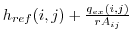
The algorithm is based on Albrecht (2011). In this scheme, if cell (![]() ) fits the criteria, a reference thickness
) fits the criteria, a reference thickness
![]() is found, defined as an average over the thickness of all neighboring cells with
is found, defined as an average over the thickness of all neighboring cells with ![]() that are contributing mass to (
that are contributing mass to (![]() ). The total mass input over the time step to (
). The total mass input over the time step to (![]() ) is calculated as
) is calculated as
![]() . This is added to the volume of ice already in the cell, which is nonzero only if
. This is added to the volume of ice already in the cell, which is nonzero only if
![]() at the beginning of the time step, and is equal to
at the beginning of the time step, and is equal to
| (6.109) |
(If
| (6.110) |
is found. If
-
 is set to 2,
 is set to
 ,
,
 is set to
 .
.
-
is set to 1,
-
is set to
,
-
is set to
 ,
,
- Excess flux
 is found.
- adjacent cells that are not completely covered (
 or 1) are searched for.
- if there are no suitable cells,
 is put back into cell (
 ) (
is set to
) (
is set to
 ).
).
- if there are suitable cells,
 is divided uniformly among the corresponding faces of the receiving cells, and the algorithm begins again.
If calve_to_mask=.true., this sets a limit to how far the front can advance, even if advance is allowed. The front will not advance into cells where the array calve_mask is not equal to 1. This mask must be set through a binary input file.
No calving parameterisation is implemented in STREAMICE. However, front advancement is a precursor for such a development to be added.
6.6.4.3.6 Surface/basal mass balance
After updating thickness in fully- and partially-covered cells, surface and basal mass balances are applied to nonempty cells. Currently surface mass balance is a uniform value, set through the parameter streamice_adot_uniform. Basal melt rates are stored in the array BDOT_streamice, but are multiplied through by float_frac_streamice before being applied.
Next: 6.7 Packages Related to Up: 6.6 Sea Ice Packages Previous: 6.6.3 SHELFICE Package Contents mitgcm-support@mitgcm.org
| Copyright © 2006 Massachusetts Institute of Technology | Last update 2018-01-23 |


