 |
 |
|||||||||||
 |
|
|||||||||||
 |
 |
|||||||||||


|
Next: 6.3.6 Tapering: Danabasoglu and Up: 6.3 Gent/McWiliams/Redi SGS Eddy Previous: 6.3.4 Variable Contents Subsections 6.3.5 Tapering and stabilityExperience with the GFDL model showed that the GM scheme has to be matched to the convective parameterization. This was originally expressed in connection with the introduction of the KPP boundary layer scheme (Large et al., 97) but in fact, as subsequent experience with the MIT model has found, is necessary for any convective parameterization.
6.3.5.1 Slope clipping
Deep convection sites and the mixed layer are indicated by
homogenized, unstable or nearly unstable stratification. The slopes in
such regions can be either infinite, very large with a sign reversal
or simply very large. From a numerical point of view, large slopes
lead to large variations in the tensor elements (implying large bolus
flow) and can be numerically unstable. This was first recognized by
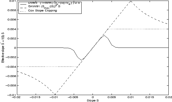
Cox, 1987, who implemented ``slope clipping'' in the isopycnal mixing
tensor. Here, the slope magnitude is simply restricted by an upper
limit:
Notice that this algorithm assumes stable stratification through the ``min'' function. In the case where the fluid is well stratified (
while in the limited regions (
so that the slope magnitude is limited The slope clipping scheme is activated in the model by setting GM_taper_scheme = 'clipping' in data.gmredi.
Even using slope clipping, it is normally the case that the vertical
diffusion term (with coefficient
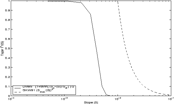
6.3.5.2 Tapering: Gerdes, Koberle and Willebrand, Clim. Dyn. 1991The tapering scheme used in Gerdes et al., 1999, ([42]) addressed two issues with the clipping method: the introduction of large vertical fluxes in addition to convective adjustment fluxes is avoided by tapering the GM/Redi slopes back to zero in low-stratification regions; the adjustment of slopes is replaced by a tapering of the entire GM/Redi tensor. This means the direction of fluxes is unaffected as the amplitude is scaled.
The scheme inserts a tapering function,
where The GKW tapering scheme is activated in the model by setting GM_taper_scheme = 'gkw91' in data.gmredi.
Next: 6.3.6 Tapering: Danabasoglu and Up: 6.3 Gent/McWiliams/Redi SGS Eddy Previous: 6.3.4 Variable Contents mitgcm-support@dev.mitgcm.org
|
||||||||||||||||||||||||||||
![$\displaystyle f_1(S) = \min \left[ 1, \left( \frac{S_{max}}{\vert S\vert}\right)^2 \right]$](img1755.png)


