Multi Scale Superparameterization in Ocean Modeling
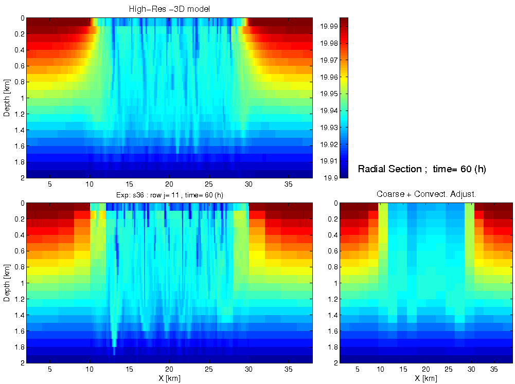
story by Helen HillMulti scale approaches allow explicit modeling of the many different phenomena that are present in the real ocean. Borrowing an idea from meteorology (that of the embedded Cloud Resolving Model), Jean Michel Campin and colleagues have been using the MITgcm to exploit a multi scale superparameterization approach to increase efficiency in modeling oceanic deep convection (ODC). Figure 1 compares cross-domain temperature sections from three runs after 2.5 days of simulation. The bottom left hand panel (from the run taking a multi scale superparameterization approach) shares much more in character with the field deriving from the fully resolved model (top left) than that from the balanced model with only a simple convective adjustment algorithm (bottom right) yet for only a modest increase in computational cost.

Figure 1. Temperature sections after 60 hours from (top left) the fully resolved model, (bottom left) the multi-scale simulation and (bottom right) the balanced model with a simple convective adjustment algorithm. The multi-scale simulation image is derived from a composite of 2-D embedded elements.
Taking an idealised but fully resolved, three-dimensional, non-hydrostatic model of ODC as their “ground-truth” solution, in this approach, multiple 2 dimensional, Plume-Resolving, non-hydrostatic Models (PRMs) are embedded in a large-scale, 3 dimensional, coarse resolution, BAlanced Model (BAM). Using tendencies from PRMs running at each horizontal grid-point of the BAM as drivers, the ESMF-exploiting coupling between PRM and BAM is two-way: the PRM receives information about the large-scale shear and temperature/salinity environment from the BAM, computes momentum and T/S tendencies by integrating forward very high resolution submodels, and then returns the tendencies to the BAM.
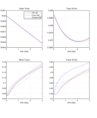
Two first questions always arise with any potential new parameterization scheme: How well does it work and how efficient is it? To demonstrate how well the embedded PRMs do, the team compared the time evolution of, among other metrics, mean temperature and passive tracer concentration and the standard deviations of each. They demonstrate (fig. 2) much closer temporal and spatial agreement for the run with the new parameterization “scheme” (in red) than that for the BAM with convective adjustment alone (the blue line). The high resolution solution is in black. Reducing the convective vertical diffusion coefficient in the convective adjustment run from 10 m²/s (unbroken blue) to 2.5m²/s (dashed blue) to match the average tracer concentration at t=3 days in the “ground-truth” solution does little to improve the tracer and temperature standard deviations in a BAM run with convective adjustment.

Figure 2. Time evolution of mean temperature (top left), temperature standard deviation (top right), mean tracer (bottom left) and tracer standard deviation (bottom right) for the high resolution model (black), the BAM with convective adjustment having a vertical diffusion coefficient of 10m²/s (unbroken blue) or 2.5m²/s (dashed blue) and the BAM with embedded plume models (red).
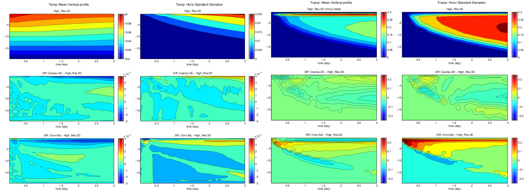
Figure 3 shows the time evolution of the vertical profiles of each quantity (the means and standard deviations of temperature and tracer) illustrating, in greater detail, the comparative temporal and spatial distributions in the three runs.

Figure 3. Evolution of vertical profiles of temperature (column 1), temperature standard deviation (column 3), tracer (column 2) and tracer standard deviation (column 4) for the three run types – fully resolved (top row), BAM with embedded PRMs (middle row) and BAM with convective adjustment (bottom row).
In terms of efficiency: the explicitly resolving, 2-D, sub-grid scale PRM is only a few times (~3-5) slower than the same model with convective adjustment but much faster (>10) than the 3-D non-hydrostatic plume resolving model.
Quantitative comparison of the fully resolved simulation, the multiscale realisation and the BAM alone (with a basic convective adjustment algorithm to represent vertical mixing), demonstrates that the new implementation does a great job, closely tracking the fully resolved non-hydrostatic model but for a far lower computational cost: By exploiting parallelism amongst the embedded models, the wall-clock time to solution is only a small multiple of that for the pure hydrostatic simulation.
Excitingly this technique could find broad applicability: Other mixed-layer processes, biogeochemical processes and eddy flux coefficients each have the potential to be estimated by a similar coupled implementation of local, prognostic, sub-models nested within a lower resolution model at larger scale. Maybe they too can realise significant increases in fidelity of the larger-scale solution for only a moderately raised computational cost.
Want to find out more? – contact Jean Michel Campin.

Jean-Michel has been working with the MITgcm since 1992. He loves biking and is a connoisseur of Belgian beer.
References:
A paper reporting this work is currently in preparation. Check back here for a draft.
EGU ’08 presentation (PDF)
