A search for multiple equilibria in a complex climate model…
story by Helen Hill

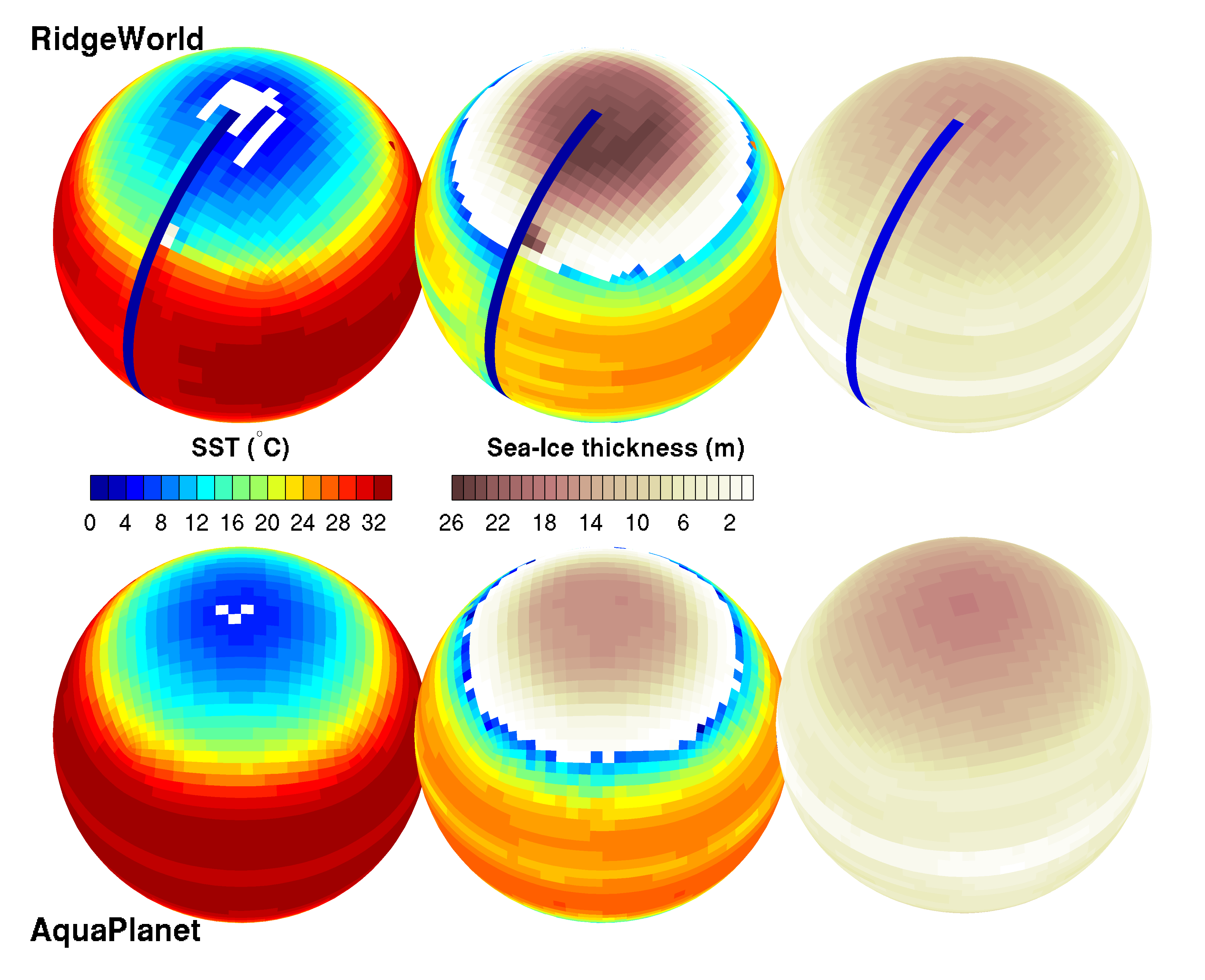
Figure 1 – SST and sea-ice thickness in Ridge (top) and Aqua (bottom) for the Warm (left), Cold (middle) and Snowball (right) states. In the Snowball state, the planet is covered with about a hundred meters of ice and thickening toward the poles. While low-order climate models have been found to exhibit multiple equilibria of the kind found by Ferreira and co-workers, this is the first time such equilibria have been revealed in a model with so many degrees of freedom… (image source – D. Ferreira, Marshall group)
This month we look at work by David Ferreira, John Marshall and Brian Rose who, prompted by earlier theoretical work on multiple equilibria (Rose and Marshall, 2009), have been using a coupled ocean-atmosphere-sea ice configuration of MITgcm to probe for multiple equilibria in a more sophisticated climate model. Although low-order energy balance models of the climate are known to exhibit intransitivity, i.e. more than one climate state for a given set of governing equations, Ferreira et al’s results are the first to demonstrate that this is a property of a complex coupled model with an energetically-consistent set of equations representing the 3d dynamics of the ocean and atmosphere (i.e., there is importantly no flux correction). Their coupled model notably includes atmospheric synoptic systems, large-scale circulation of the ocean, a fully active hydrological cycle, sea-ice and a seasonal cycle.
Multiple Equilibria
A central question in climate research concerns the existence, or otherwise, of multiple equilibria. Lorenz (1968, 1970) discusses the implications for climate of whether the governing equations are transitive, supporting only one set of long-term statistics, or whether they are intransitive, supporting two or more sets of long-term statistics (i.e. multiple equilibria), each of which has a finite probability of resulting from random initial conditions. The proven existence of multiple equilibria would have a profound impact on our interpretation of the paleoclimate record and our perspectives on possible future climates. In the context of global climate change in response to anthropogenic greenhouse gas emissions, for example, if multiple equilibria exist then the possibility of massive (and possibly abrupt) climate shifts in response to slow changes, would have to be taken very seriously, even if the chance of such an event were very unlikely. Moreover, if the levels of atmospheric greenhouse gases were to be reduced, the climate might not necessarily return to its prior state.
In an attempt to exploit the information and knowledge encoded in coupled climate models, Marshall’s group has been using them to explore some of the basic questions in climate such as what sets the pole-equator temperature gradient and the extent of polar ice caps – see for instance Modeling Water Worlds (March, 2009) and The Role of Ocean Circulation in Atlantic Decadal Variability (May, 2010). In particular the team has been studying partition of energy transport, and the extent of polar ice, in highly idealized worlds in which there is no land, or the land distribution is highly idealized comprising meridional barriers with and without gaps, so-called Aquaplanets. It is in this context that they have been able to identify three different stable states for exactly the same set of parameters and external forcings: a cold state in which a polar sea-ice cap extends into midlatitudes, a warm state which is ice-free and a completely sea ice covered `Snowball’ state. While low-order climate models have been found to exhibit multiple such equilibria, this is the first time they have been revealed in a model with so much realistic interior variability. This variability emerges from weather systems (atmospheric turbulence) and seasonal fluctuations of the solar forcing and interactions between the climate components (ocean, atmosphere, and sea ice).
The following movie illustrates the behavior of the MITgcm Aquaplanet system as it is driven from a warm ice-free state to a Snowball (completely ice-covered) state by a linearly decreasing solar constant. The top panel shows the Sea Surface Temperature (color) and sea ice cover (white). The bottom panel shows the evolution of the solar constant and the average latitude of the sea ice edge as a function of time. The presence of multiple equilibrium states is revealed in the evolution of the sea ice edge which does not follow a linear trend. Rather, the ice edge “sticks” around the equilibrium positions for decades and abruptly transition between positions (Animation credit: David Ferreira, Marshall Group, MIT)
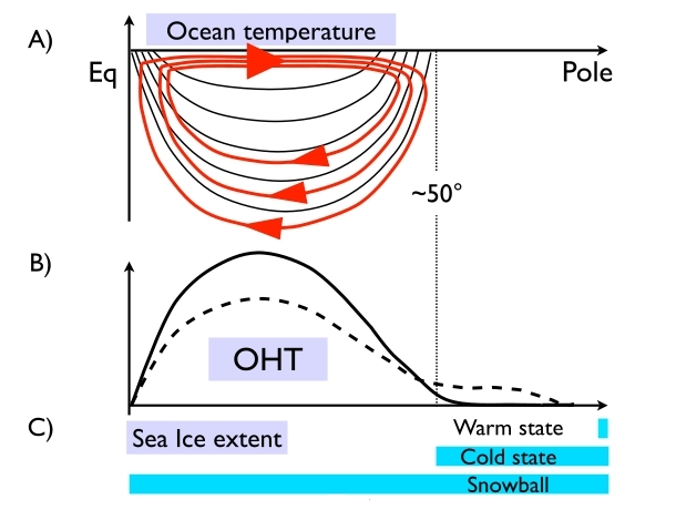
The key characteristics of the multiple states found by Ferreira, Marshal and Rose, and seen in the movie above, are summarized in the diagram shown in figure 2.

Figure 2 – Schematic of the multiple states observed by Ferreira, Marshall and Rose: A) shows the thermal structure of the ocean (in black) with the residual overturning circulation (superimposed in red), B) the Ocean Heat Transport (OHT) in the Warm (dashed) and Cold (solid) states, and C) sea ice extent for the 3 stable states. All curves are plotted against latitude with the Equator to the left and the Pole to the right.(image source D Ferreira, Marshall Group)
This schematic shows the ocean’s thermocline, residual circulation, ocean heat transport and sea-ice extent in the Warm, Cold and Snowball states. The latitude of 50o corresponds (approximately) to the poleward edge of the subtropical thermocline set by the pattern of prevailing winds. Since the multiple equilibria exist in both Ridge and Aqua, the schematic emphasizes their common aspects. Further analysis of the simulations and theoretical work based on Rose and Marshall (2009) showed that the characteristic shape of the OHT shown in Fig. 2 is key to the existence of the 3 multiple states. Interestingly, such a shape is observed on Earth today and seen in a wide variety of climate simulations. The Warm climate is as warm as the Eocene (around 50M years ago), with little or no ice and abyssal ocean temperatures which are very warm (15oC in Aqua, 7oC in Ridge). The Cold climate has extensive ice caps and abyssal temperatures hovering around 0oC.
Using MITgcm to model climate
Exploiting MITgcm’s between ocean and atmosphere dynamics to generate a coupled atmosphere and ocean model with a shared dynamical core (Marshall et al. 2004), the model uses the rescaled height coordinate Z* for the Boussinesq ocean (Adcroft and Campin, 2004). As described in Adcroft et al. 2004, both atmosphere and ocean use the same cubed-sphere grid with 24 x 24 points per face to yield a resolution of 3.75o at the equator. Besides avoiding problems associated with converging meridians at the poles, use of such a grid greatly simplifies implementation of a conservative atmosphere-oceans interface (Campin et al. 2008).
The atmospheric model is based on the SPEEDY physics scheme (Molteni, 2003). Briefly it includes a 4-band radiation scheme, a parameterization of moist convection, diagnostic clouds and a boundary layer scheme. Vertical resolution is low with one level in the boundary layer, three in the troposphere and one in the stratosphere.
The 3km deep, flat-bottomed ocean model has 15 vertical levels, increasing from 30m at the surface to 400m at depth. The model uses GM mixing and isopycnal diffusion, both with a transfer coefficient of 1200m2s-1. Convective adjustment, implemented as an enhanced vertical mixing of temperature and salinity, is used to represent ocean convection. The background vertical diffusion is uniform and set to a value of 3x 10⁻⁵ m2s-1. The model uses a non-linear equation of state. Sea-ice is modelled based on the Winton (2000) two and a half layer thermodynamic model. Prognostic variables are ice fraction, snow and ice thickness, and a two-level enthalpy representation which accounts for brine pockets and sea-ice salinity, employing an energy conserving formulation. The model uses diffusion of sea ice thickness as a proxy of sea-ice dynamics. The snow albedo parameterization depends on snow height, surface temperature and age. The atmospheric CO2 level is prescribed at present levels. The seasonal cycle insolation is represented but there is no diurnal cycle. The set up is identical to that used in Ferreira et al (2010).
Fluxes of of momentum, freshwater, heat and salt are exchanged every hour (the ocean time-step). Finally, by using the Z* coordinate, (Campin et al., 2008), the model requires no artificial limit of sea ice thickness to avoid drying out of ocean cells, therefore allowing a realistic treatment of the sea ice-ocean interface. The model is shown to achieve perfect (to machine-accuracy) conservation of freshwater, heat and salt during extended climate simulations, a key property of the fidelity and integrity of the coupled system.
The model includes atmospheric synoptic systems, a large-scale ocean circulation, a fully active hydrological cycle (evaporation and precipitation), snow and sea-ice as well as a seasonal cycle. There are no flux adjustments, the system being solely forced by incoming solar radiation at the top of the atmosphere.
Future Explorations…
The team is currently investigating the stability of the multiple equilibria and likely mechanisms of transition from one to the other and overlaying models of the carbon cycle and the partition of carbon between atmospheric and oceanic reservoirs.
References:
Adcroft, A., J.M. Campin, C. Hill, and J. Marshall, 2004: Implementation of an Atmosphere-Ocean General Circulation Model on the Expanded Spherical Cube. Mon. Wea. Rev., 132, 2845-2863. doi:10.1175/MWR2823.1
Adcroft, A., and J.-M. Campin, 2004: Re-scaled height coordinates for accurate representation of free-surface flows in ocean circulation models. Ocean Model., 7, 269-284. doi:10.1016/j.ocemod.2003.09.003
Campin, J.-M., J. Marshall, and D. Ferreira, 2008: Sea ice-ocean coupling using a rescaled vertical coordinate Z* . Ocean Model., 24, 1-14. doi:10.1016/j.ocemod.2008.05.005
Ferreira, D., J. Marshall, and J.-M. Campin, 2010: Localization of Deep Water Formation: Role of Atmospheric Moisture Transport and Geometrical Constraints on Ocean Circulation. J. Climate. 23, 1456-1476. doi:10.1175/2009JCLI3197.1
Marshall, J., A. Adcroft, J.M. Campin, C. Hill, and A. White, 2004: Atmosphere-Ocean Modeling Exploiting Fluid Isomorphisms. Mon. Wea. Rev., 132, 2882-2894. doi:10.1175/MWR2835.1
Molteni, F., 2003: Atmospheric simulations using a GCM with simplified physical parametrizations. I: model climatology and variability in multi-decadal experiments. Clim. Dyn., 64, 175-191. doi:10.1007/s00382-002-0268-2
Rose, B. and J. Marshall, 2009: Ocean heat transport, sea-ice and multiple climate states: insights from energy balance models. J. Atmos. Sci., 66, 9, 2828-2843. doi:10.1175/2009JAS3039.1
Winton, M., 2000: A Reformulated Three-Layer Sea Ice Model. J. Atmos. Oceanic Technol., 17, 525-531. doi: 10.1175/1520-0426(2000)017<0525:ARTLSI>2.0.CO;2
